The following images are taken from DesignCrowd.

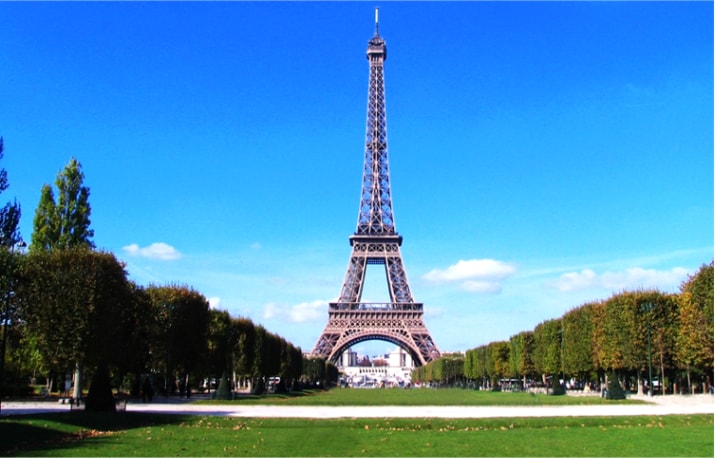
This first image is an image with tourists ( I call it as tour) while the second one has no tourist – no_tour.
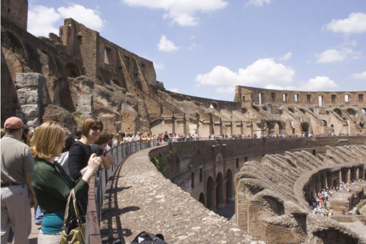 This is another
 new image that is different from the above two.
The goals are:
- Use PCA to compress the
tourimage - Test the generalizability of the PC loadings obtained from
tourimage to other similar image (i.e., theno_tourimage) and a very different image (i.e.newimage).
Loading pictures and standardizing the sizes
First, let’s load the pictures and look at the dimensions.
library(jpeg)
path = "C:/Users/mirac/Desktop/Work/acadblog2/static/img/imagecompression"
tour = readJPEG(paste(path,"paris_tourist.jpg", sep = "/"))
no_tour = readJPEG(paste(path,"paris_no_tourist.jpg", sep = "/"))
new = readJPEG(paste(path,"rome.jpg", sep = "/"))
dim(tour); dim(no_tour); dim(new)## [1] 459 715 3## [1] 458 715 3## [1] 500 750 3The three pistures do not have the same dimensions so let’s resize them to 458, 715, 3. The 3 represents R, G, and B, the three color schemes from the images.
library("EBImage")
# scale to a specific width and height
tour <- resize(tour, w = 458, h = 715)
new <- resize(new, w = 458, h = 715)

# extract the pixel array
tour <- as.array(tour)
new <- as.array(new)
The tour Image.
PCA
Break down each color scheme into three dataframe and perform PCA.
rtour = tour[, ,1]
gtour = tour[, ,2]
btour = tour[, ,3]
prtour = prcomp(rtour, center = FALSE)
pgtour = prcomp(gtour, center = FALSE)
pbtour = prcomp(btour, center = FALSE)
tour.pca = list(prtour, pgtour, pbtour)Scree Plot and Cumulative Variation Plot
Take a look at the Scree plot of the PCA.
library(dplyr)
# Create a dataframe for easier plotting
df = data.frame(scheme = rep(c("R", "G", "B"),each =458),
                index = rep(1:458,  3),
                var = c(prtour$sdev^2,
                        pgtour$sdev^2,
                        pbtour$sdev^2))

df %<>% group_by(scheme) %>%
  mutate(propvar =100*var/sum(var)) %>%
  mutate(cumsum = cumsum(propvar)) %>%
  ungroup()

#plot
library(ggplot2)
#relevel to make it look nicer
df$scheme = factor(df$scheme,levels(df$scheme)[c(3,2,1)])

df %>% ggplot(aes( x = index, y = propvar, fill = scheme)) +
    geom_bar(stat="identity") +
    labs(title="Screeplot of Principal Component", x ="Principal Component",
         y="% of Variance") + geom_line()  +
    scale_x_continuous(limits = c(0,30)) +
    facet_wrap(~scheme)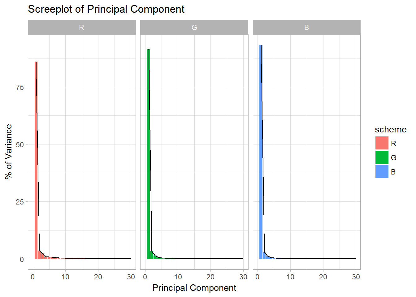
Figure 1: The elbow of the screeplot is between the fourth and the fifth PC
df %>% ggplot(aes( x = index, y = cumsum, fill = scheme)) +
    geom_bar(stat="identity") +
    labs(title="Cumulative Proportion of Variance Explained Principal Component", x="Principal Component",
         y="Cumulative % of Variance") + geom_line() +
    scale_x_continuous(limits = c(0,30)) +
    facet_wrap(~scheme)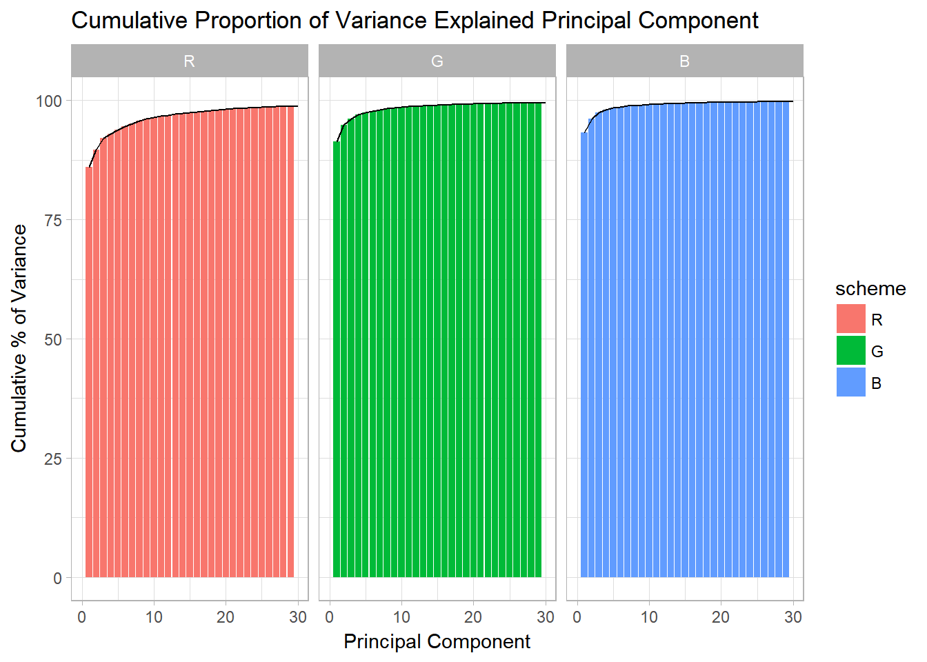
Figure 2: Thirty PCs appear to be good enough to explain most of the variations
It seems like the first 30 PCs have enough proportion of variance covered because the proportion of variance explained is close to 100%.
Image Reconstruction
Let’s reconstruct the first image. I choose to look at the images constructed from 2, 30, 200, and 300 Prinicipal Components.
# This is the number of desired PCs
pcnum = c(2,30,200, 300)

for(i in pcnum){
    pca.img <- sapply(tour.pca, function(j) {
      compressed.img <- j$x[,1:i] %*% t(j$rotation[,1:i])
    }, simplify = 'array')
  writeJPEG(pca.img, paste(path,"/tour/tour_compressed_", round(i,0), '_components.jpg', sep = ''))
}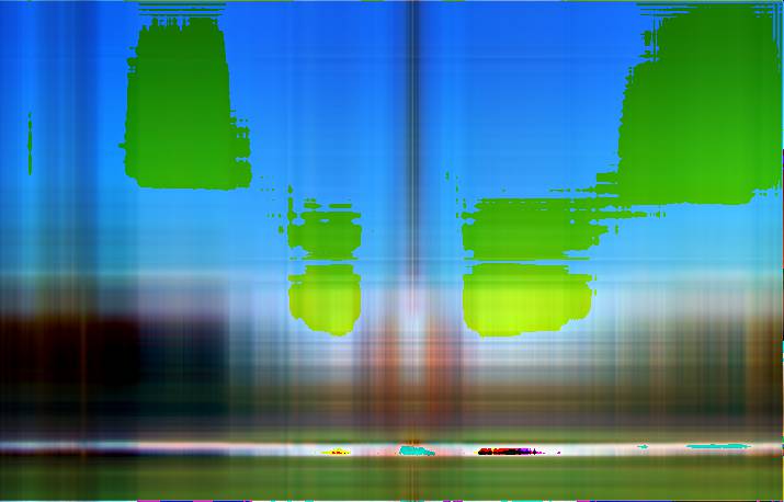
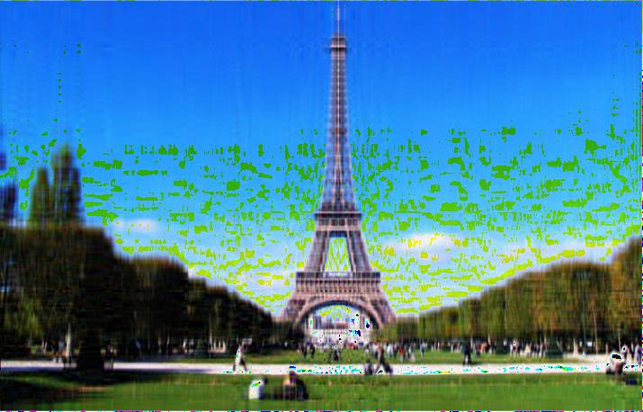

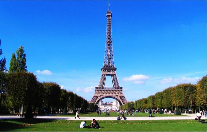
Figure 3: Compress images using 2, 30, 200 and 300 PCs respectively.
It appears that using 200 PCs is enough to compress the image while maintaining a good quality.
Image Size Compression
But how about the sizes of these images?
original <- file.info(paste(path,"paris_tourist.jpg", sep ="/"))$size / 1000

for(i in pcnum){
  filename = paste("tour_compressed_",i,'_components.jpg', sep = '')
  full.path = paste(path,"tour",filename,sep = "/")
  size = file.info(full.path)$size/1000
  cat(filename, 'size:',size,"\n",
      "Reduction from the original image: ",(original-size)/original*100,"% \n\n" )
}
## tour_compressed_2_components.jpg size: 30.258
## Reduction from the original image: 53.07237 %
##
## tour_compressed_30_components.jpg size: 55.743
## Reduction from the original image: 13.54726 %
##
## tour_compressed_200_components.jpg size: 43.244
## Reduction from the original image: 32.93216 %
##
## tour_compressed_300_components.jpg size: 39.435
## Reduction from the original image: 38.8396 %Surprisingly, the compressed image that uses 30 PCs has the lowest reduction of image size.
The no_tour Image
Now, let’s use a similar image (no_tour) and use the Principal Loadings obtained from the previous step to execute image compression.
The compress () function is meant for compressing a new image (i.e., image not used in the previous step to obtain Principal Loadings).
rno_tour = no_tour[, ,1]
gno_tour = no_tour[, ,2]
bno_tour = no_tour[, ,3]

no_tour_rgb = list(rno_tour,gno_tour,bno_tour)

compress <- function(trained_rgb_pca, newrgb, pcnum, dims){
   r_rotate = trained_rgb_pca[[1]]$rotation
   g_rotate = trained_rgb_pca[[2]]$rotation
   b_rotate = trained_rgb_pca[[3]]$rotation

   r = newrgb[[1]]
   g = newrgb[[2]]
   b = newrgb[[3]]

  pred_r = (r %*% r_rotate)[,1:pcnum] %*% t(r_rotate[,1:pcnum])
  pred_g = (g %*% g_rotate)[,1:pcnum] %*% t(g_rotate[,1:pcnum])
  pred_b = (b %*% b_rotate)[,1:pcnum] %*% t(b_rotate[,1:pcnum])

  pred.pca = list(pred_r, pred_g, pred_b)
  pred.array = array(as.numeric(unlist(pred.pca)),dim = dims)
  return(pred.array)
}

for(i in pcnum){
    pca.img = compress(tour.pca, no_tour_rgb, pcnum = i, dims = c( 458, 715,3))
    writeJPEG(pca.img, paste(path,"/no_tour","/no_tour_compressed_", round(i,0), '_components.jpg', sep = ''))
}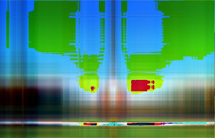
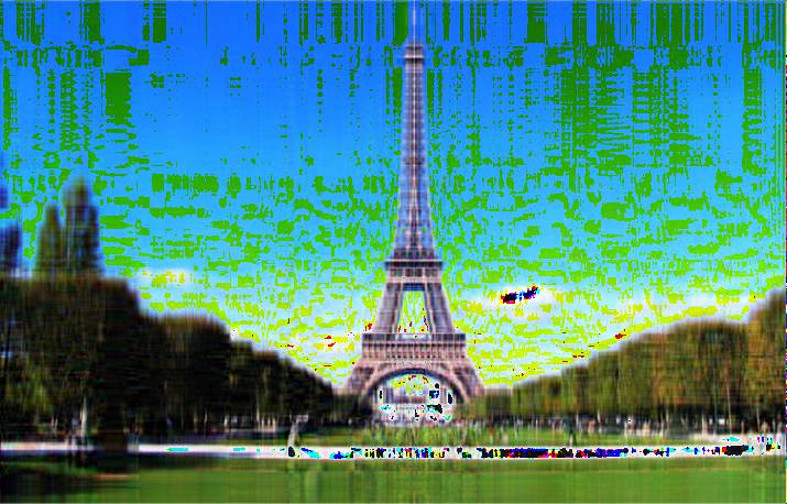
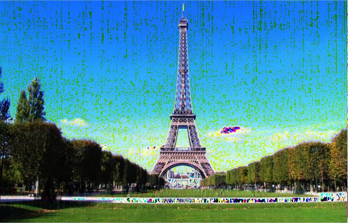
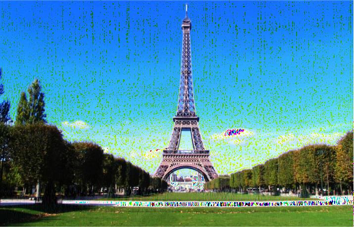
Figure 4: Compress simialr images to test the generalizability of PCs
One can observe that the last image’s quality is the best out of four (since it uses the most PCs) but it is not even close to a high quality image.
The new Image.
We now know that the performance of PCA in image compression is highly useful to its original image but not for a similar image. It’s natural to ask whether it will be worst if a totally unrelated image (such as new image) was used instead. Let’s check it out.
rnew = new[, ,1]
gnew = new[, ,2]
bnew = new[, ,3]

new_rgb = list(rnew,gnew,bnew)

for (i in pcnum){
    pca.img = compress(tour.pca, new_rgb, pcnum = i, dims = c(458,715, 3))
    writeJPEG(pca.img, paste(path,"/new","/new_compressed_", round(i,0), '_components.jpg', sep = ''))
}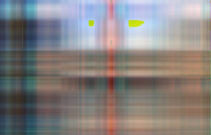
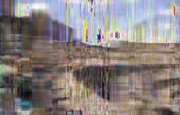
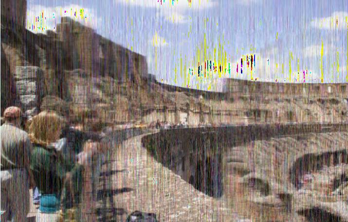
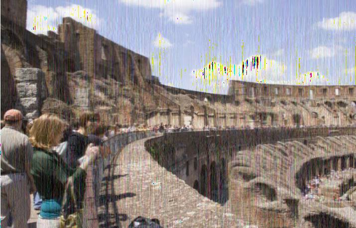
Figure 5: Compressing a non-related image using previously extracted PC loadings
While the image output does not look exactly like the original image, the main features of the image is clearly shown on it. This is pretty impressive because the machine learns the rules of extracting important information based on only one image tour. One can experiment increase the number of PCs to get a higher resolution image too.
Summary
Principal Component Analysis is a great tool for dimension reduction (thus, sinze reduction in this case), extracting important insights, and uncover underlying message of a dataset.