Missing data, NAs

# Explore the NAs
#Make a copy of dataset for that
dat_NA = full_dat
# Substitute unknowns in the dataset with NA
dat_NA[dat_NA == "unknown"] <- NA

library(VIM)
aggr_plot <- aggr(dat_NA, col = c('cornflowerblue','firebrick1'), numbers = TRUE, sortVars = TRUE, labels = names(full_dat), cex.axis = .7, gap = 3, ylab = c("Proportion of missing data","Maps"))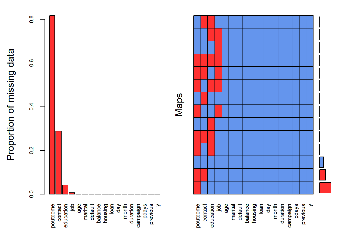

Figure 1: Distribution of NA in the dataset.

## 
##  Variables sorted by number of missings: 
##   Variable       Count
##   poutcome 0.817478047
##    contact 0.287983013
##  education 0.041074075
##        job 0.006370131
##        age 0.000000000
##    marital 0.000000000
##    default 0.000000000
##    balance 0.000000000
##    housing 0.000000000
##       loan 0.000000000
##        day 0.000000000
##      month 0.000000000
##   duration 0.000000000
##   campaign 0.000000000
##      pdays 0.000000000
##   previous 0.000000000
##          y 0.000000000

About 80% of the predictor poutcome, 30% of predictor contact, 4% of predictor education and 0.6% of predictor job have missing data (see Figure 1). There will be 37369 rows that had to be deleted if rowwise NA deletion was executed. The other way is to remove entirely those variables that contains NA including poutcome, contact, education and job. However, this is not desirable because we dont know whether those variables are important or not. In short, deletion is not an ideal way.

This leads to another possibility: Imputation. One of the easiest way is to use the KNN Imputation. This algorithm identifies k closest observations to the to-be-imputed observation and take the weighted average based on the distance. Yet, imputing ~ 80% of the data for poutcome variable is not sensible at all.

Since all of the missing data exist at categorical data, the strategy used was to treat the “unknown” as a category itself (pg 332 ESL II).

Imbalance Classification

counts <- table(full_dat$y)
barplot(counts,col = c("darkblue","red"),legend = rownames(counts), main = "Term Deposit")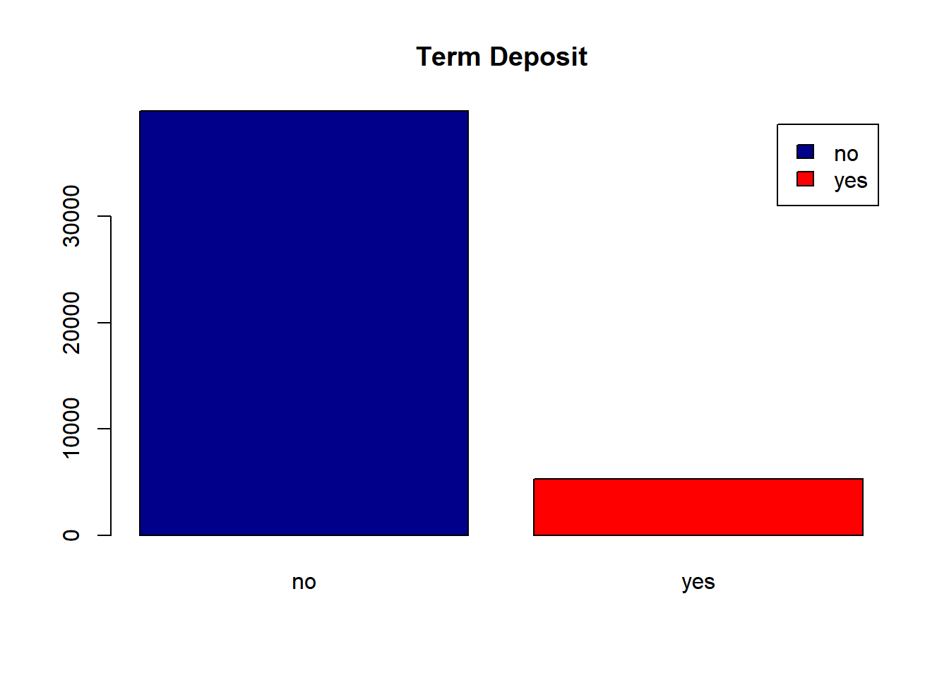

Figure 2: Proportion of responses: Yes or No

Due to the highly imbalance of the proportion of responses (as shown in Figure 2, and due to large sample size of 45211, the dataset was subsetted at random with controlling the proportion of responses to be equal. This process is known as undersampling. From there, a dataset of size N = 2130 was drawn at random.

N = 2130
# Subset the data to "Yes" responses and "No" responses
yes_dat <- full_dat[full_dat$y == "yes",]
no_dat <- full_dat[full_dat$y == "no",]

# sampling for the index that will be used to pick the observations
set.seed(1001)
yes_index = sample(1:nrow(yes_dat), N/2)
no_index = sample(1:nrow(no_dat), N/2)

# Extracting the data
dat <- rbind(yes_dat[yes_index,], no_dat[no_index,])

The previous process is very important to be done or a simply “prediction” of NO to subscription would yield 0.88 % of accuracy in this dataset. This undersampled data set is referred as “dataset” from now on.

Correlation

The correlation between the numeric features were looked into too.

#Numeric data columns
nume_col = c(1,6,10, 12:15)
pearson = cor(dat[,nume_col])
library(corrplot)
corrplot(pearson, type = "upper")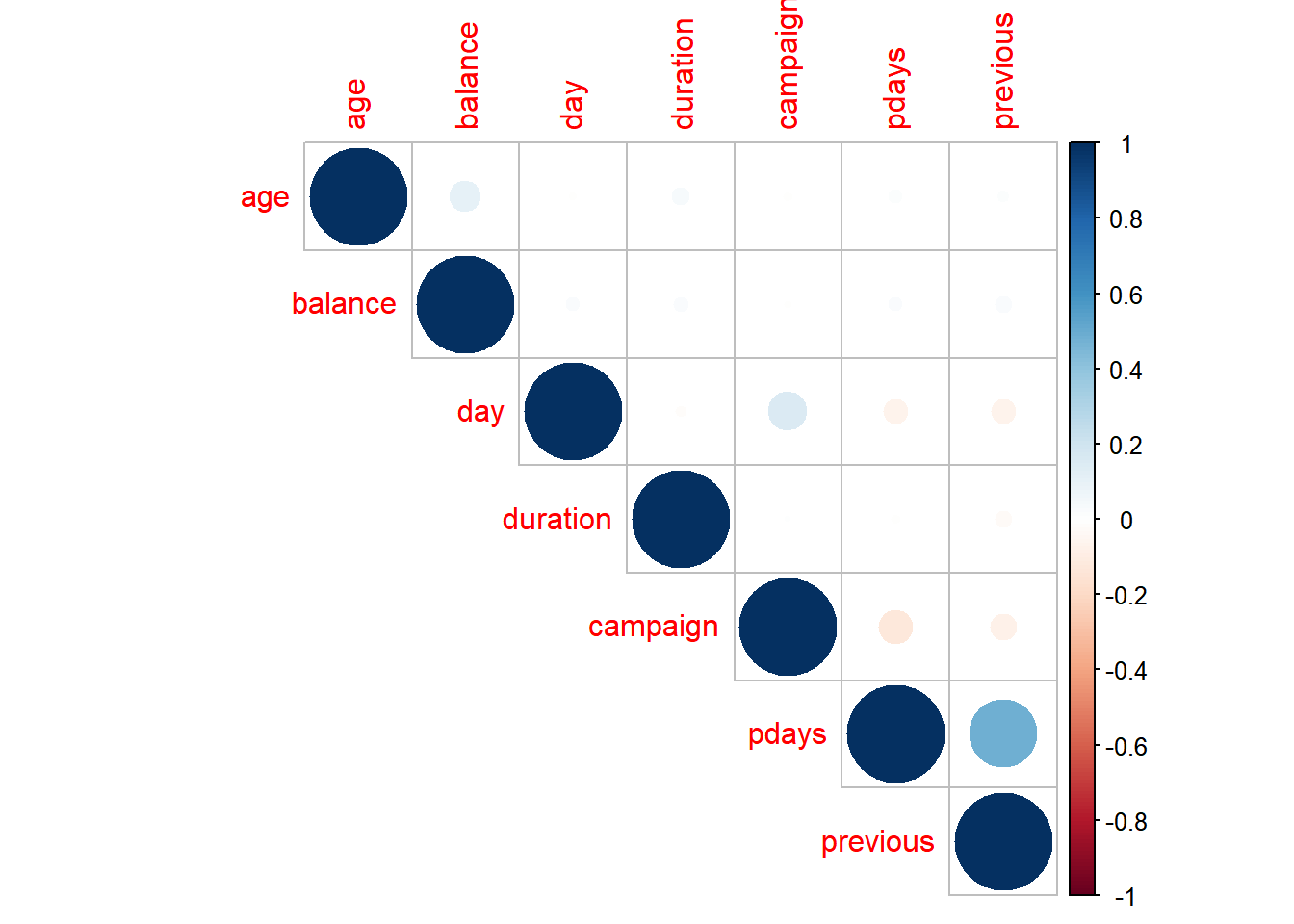

Figure 3: Correlation between numerical predictors.

Through visual inspection of Figure 3, it was found that the Pearson’s correlation between predictors are low except the one for features previous and pdays. The Pearson’s correlation is 0.48. Why is that so?

It was described at [Moro et al., 2011] that:

• pdays: number of days that passed by after the client was last contacted from a previous campaign (-1 means client was not previously contacted)
• previous: number of contacts performed before this campaign and for this client

This explains the high correlation between the two variables.

Distributions

The predictors balance, duration, and pdays have large standard deviations, as shown at the following.

apply(dat[,nume_col],2,sd)

##         age     balance         day    duration    campaign       pdays    previous 
##   12.005758 3300.296919    8.476752  349.509259    2.588204  102.240956    2.745466

The distributions of each features and response is shown in Figure 4. It can be seen that the distributions of predictors balance, duration, campaign, pdays, and previous are highly skewed.

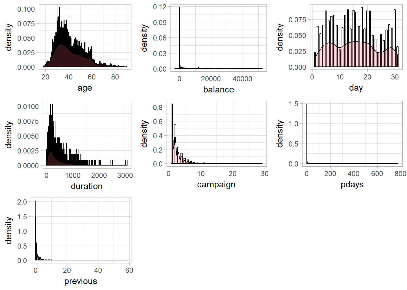
Figure 4: Histograms and Kernel density esimates of Numerical predictors

Training and Testing Data

The dataset was then split half into training and testing dataset.

# Splitting test and train data
set.seed(1001)
train = sample(1:nrow(dat), N/2)
test = -train
x.test = dat[test,-17]; y.test = dat[test,]$y

Decision Tree fitting

Decision Tree (DT) was used to fit the data. Decision Tree breaks the space of the data into partitions and predict the value by taking the average of each partitions. The rule of dividing the model space is specified by minimizing the classification error rate and while controlling the size of the tree (i.e., number of terminal nodes). The following image is obtained from ISL.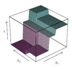

library(tree)
# Fitting tree
treemod = tree(y ~., subset = train, data = dat)
sum_tree = summary(treemod)
err_tree = sum_tree$misclass[1]/sum_tree$misclass[2]

The error of misclassification was 0.1802817. However, this is the traning error rate and it could be biased.

Cross-validation, Tree-pruning and Training Errors

Cross-validation was used to choose the best number of terminal nodes and the decision tree was pruned.

set.seed(1001)
cvtree = cv.tree(treemod ,FUN = prune.misclass )
choose_nodes = cbind(cvtree$size, cvtree$dev)
colnames(choose_nodes) = c("Number of terminal nodes", "CV error")
choose_nodes

##      Number of terminal nodes CV error
## [1,]                       12      248
## [2,]                       10      248
## [3,]                        8      244
## [4,]                        7      247
## [5,]                        4      273
## [6,]                        2      312
## [7,]                        1      818

plot(cvtree$size ,cvtree$dev ,type = "b", xlab = "Number of terminal nodes", ylab = "cross-validation error", col = "purple4")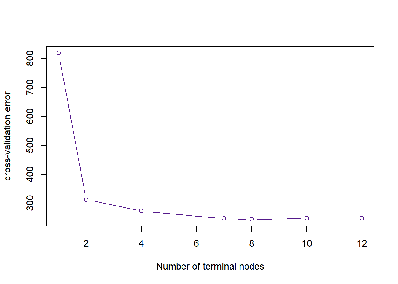

Figure 5: The cross-validation error rate across the number of terminal nodes

As shown in Figure 5, the best number of terminal nodes was 8 because it gives the lowest CV errors. The tree was pruned accordingly.

prunetree = prune.misclass(treemod ,best = 8)
sum_prune= summary(prunetree)
err_prune = sum_prune$misclass[1]/sum_prune$misclass[2]
cbind(err_tree, err_prune)

##       err_tree err_prune
## [1,] 0.1802817 0.1849765

The misclassification error of pruned tree is higher in this case. However, note that this is just a training error.

Testing Error and Prediction Accuracy

The testing error was inspected too.

# Test Performance
tree.pred = predict (prunetree , x.test ,type="class")
table(tree.pred, y.test)

##          y.test
## tree.pred  no yes
##       no  414  85
##       yes 130 436

The confusion error above shows that the fitted tree tends to predict a Yes response to term subscriptiion. The testing error rate was 0.202. In other words, the prediction accuracy was 0.798.

Interpretation

The visualization of decision tree is shown below.

plot(prunetree)
text(prunetree ,pretty = 0)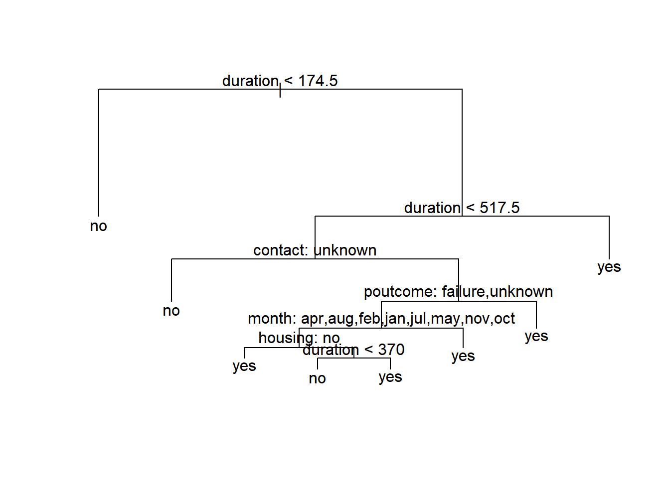

Figure 6: Visualization of decision tree.

The key variables shown in Figure 6 are:

• duration: last contact duration, in seconds
• contact: contact communication type (“unknown”, “telephone”, “cellular”)
• poutcome: outcome of the previous marketing campaign (“unknown”,“other”,“failure”,“success”)
• month: last contact month of year
• housing: has housing loan? (yes or no)

The decision tree predicts that when the representative contacted the client for more or equal to 692 (174.5+517.5) seconds on last phone call, the client would subscribe for the term deposit. If the last contact duration is less than 174.5 seconds, the client would reject the offer.

If the previous contact duration is between 174.5 and 517.5 seconds, and the contact communication type is unknown, the model predicts a NO to the subscription. One can interpret this as the reluctants of the bank representatives to record the communication type since they were rejected.

If the communication type was known, and the previous marketing outcomes were “failure” or “unknown”, it is predicted that the client would subscribe to the term deposit. This make sense because it is less likely for a person to subscribe twice.

Interestingly, if the the previous marketing outcomes were “success” or “other”, it’s likely that the client would subscribe if the phone call was made at the end of last quarter (i.e., March, June, September and December).

The model further predicts that the marketing campaign would success if the client had no housing loan. Yet, it is possible to persuade the client to subscribe to the term deposit if the last contact duration was longer than 370 seconds.