** This post is heavily based on R for Data Science. Please consider to buy that book if you find this post useful.**
The tibble package is part of the tidyverse package.
library (tidyverse)Creating Tibbles
Coerce into tibble using as.tibble
Most other R packages use regular data frames, so you might want to coerce a data frame to a tibble. You can do that with as.tibble():
as.tibble(iris)## # A tibble: 150 x 5
## Sepal.Length Sepal.Width Petal.Length Petal.Width Species
## <dbl> <dbl> <dbl> <dbl> <fct>
## 1 5.10 3.50 1.40 0.200 setosa
## 2 4.90 3.00 1.40 0.200 setosa
## 3 4.70 3.20 1.30 0.200 setosa
## 4 4.60 3.10 1.50 0.200 setosa
## 5 5.00 3.60 1.40 0.200 setosa
## 6 5.40 3.90 1.70 0.400 setosa
## 7 4.60 3.40 1.40 0.300 setosa
## 8 5.00 3.40 1.50 0.200 setosa
## 9 4.40 2.90 1.40 0.200 setosa
## 10 4.90 3.10 1.50 0.100 setosa
## # ... with 140 more rowsNew tibble from individual vectors using tibble()
tibble(
  x = 1:5,
  y = 1,
  z = x ^ 2 + y
)
## # A tibble: 5 x 3
## x y z
## <int> <dbl> <dbl>
## 1 1 1. 2.
## 2 2 1. 5.
## 3 3 1. 10.
## 4 4 1. 17.
## 5 5 1. 26.Observe that the input 1 in column y is repeated.
tibble() never changes the type of inputs (i.e, changes strings into factors), never changes the names of the variables, and never create row names, as compared to data.frame.
Nonsyntactic column names in tibble
It’s possible for a tibble to have column names that are not valid R variable names, aka nonsyntactic names. To refer to these variables, you need to surround them with backticks, `:
tb <- tibble(
  `:)` = "smile",
  ` ` = "space",
  `2000` = "number"
)
tb
## # A tibble: 1 x 3
## `:)` ` ` `2000`
## <chr> <chr> <chr>
## 1 smile space numberYou’ll also need the backticks when working with these variables in other packages, like ggplot2,dplyr, and tidyr.
Rename column names using rename()
new_tb = rename(tibble, new_col_name = old_col_name, ...). For example,
tb_new <- rename(tb, smile = `:)`, space = ` `)
tb_new
## # A tibble: 1 x 3
## smile space `2000`
## <chr> <chr> <chr>
## 1 smile space numberData Entry with transposed tibble: tribble()
tribble()` is customized for data entry in code: column headings are defined by formulas (i.e., they start with ~), and entries are separated by commas. This makes it possible to lay out small amounts of data in easy-to-read form:
tribble(
  ~x, ~y, ~z,
  #--|--|----
  "a", 2, 3.6,
  "b", 1, 8.5
)
## # A tibble: 2 x 3
## x y z
## <chr> <dbl> <dbl>
## 1 a 2. 3.60
## 2 b 1. 8.50A comment is added to make it clear where the column header is.
Convert vectors or lists to two-column data frames using enframe
enframe(x, name = "name", value = "value")
Example:
# natural sequence, unnamed vectors
enframe(1:3)
## # A tibble: 3 x 2
## name value
## <int> <int>
## 1 1 1
## 2 2 2
## 3 3 3## named sequence
enframe(c(a = 5, b = 7))## # A tibble: 2 x 2
## name value
## <chr> <dbl>
## 1 a 5.
## 2 b 7.enframe(c(a = 1, b = 2, c = 3))## # A tibble: 3 x 2
## name value
## <chr> <dbl>
## 1 a 1.
## 2 b 2.
## 3 c 3.Tibbles Versus data.frame
There are two main differences in the usage of a tibble versus a classic data.frame: printing and subsetting.
Printing
Tibbles are designed so that you don’t accidentally overwhelm your console when you print large data frames. It only shows the first 10 rows, and all the columns that fit on screen. In addition to its name, each column reports its type.
tibble(
  a = lubridate::now() + runif(1e3) * 86400,
  b = lubridate::today() + runif(1e3) * 30,
  c = 1:1e3,
  d = runif(1e3),
  e = sample(letters, 1e3, replace = TRUE)
)
## # A tibble: 1,000 x 5
## a b c d e
## <dttm> <date> <int> <dbl> <chr>
## 1 2018-07-10 01:58:26 2018-08-07 1 0.751 m
## 2 2018-07-09 14:09:06 2018-07-17 2 0.503 c
## 3 2018-07-10 05:34:49 2018-07-27 3 0.388 z
## 4 2018-07-09 20:07:05 2018-08-01 4 0.520 n
## 5 2018-07-10 04:54:28 2018-07-24 5 0.351 g
## 6 2018-07-09 21:16:36 2018-08-04 6 0.504 r
## 7 2018-07-09 10:23:43 2018-07-13 7 0.419 i
## 8 2018-07-09 10:19:01 2018-07-23 8 0.260 c
## 9 2018-07-09 19:16:31 2018-08-02 9 0.216 v
## 10 2018-07-10 07:01:25 2018-07-19 10 0.341 e
## # ... with 990 more rowsDisplay n rows and all columns using print()
Use print(n = , width = Inf) to display n rows and display all columns.
nycflights13::flights %>%
  print(n = 10, width = Inf)
## # A tibble: 336,776 x 19
## year month day dep_time sched_dep_time dep_delay arr_time
## <int> <int> <int> <int> <int> <dbl> <int>
## 1 2013 1 1 517 515 2. 830
## 2 2013 1 1 533 529 4. 850
## 3 2013 1 1 542 540 2. 923
## 4 2013 1 1 544 545 -1. 1004
## 5 2013 1 1 554 600 -6. 812
## 6 2013 1 1 554 558 -4. 740
## 7 2013 1 1 555 600 -5. 913
## 8 2013 1 1 557 600 -3. 709
## 9 2013 1 1 557 600 -3. 838
## 10 2013 1 1 558 600 -2. 753
## sched_arr_time arr_delay carrier flight tailnum origin dest air_time
## <int> <dbl> <chr> <int> <chr> <chr> <chr> <dbl>
## 1 819 11. UA 1545 N14228 EWR IAH 227.
## 2 830 20. UA 1714 N24211 LGA IAH 227.
## 3 850 33. AA 1141 N619AA JFK MIA 160.
## 4 1022 -18. B6 725 N804JB JFK BQN 183.
## 5 837 -25. DL 461 N668DN LGA ATL 116.
## 6 728 12. UA 1696 N39463 EWR ORD 150.
## 7 854 19. B6 507 N516JB EWR FLL 158.
## 8 723 -14. EV 5708 N829AS LGA IAD 53.
## 9 846 -8. B6 79 N593JB JFK MCO 140.
## 10 745 8. AA 301 N3ALAA LGA ORD 138.
## distance hour minute time_hour
## <dbl> <dbl> <dbl> <dttm>
## 1 1400. 5. 15. 2013-01-01 05:00:00
## 2 1416. 5. 29. 2013-01-01 05:00:00
## 3 1089. 5. 40. 2013-01-01 05:00:00
## 4 1576. 5. 45. 2013-01-01 05:00:00
## 5 762. 6. 0. 2013-01-01 06:00:00
## 6 719. 5. 58. 2013-01-01 05:00:00
## 7 1065. 6. 0. 2013-01-01 06:00:00
## 8 229. 6. 0. 2013-01-01 06:00:00
## 9 944. 6. 0. 2013-01-01 06:00:00
## 10 733. 6. 0. 2013-01-01 06:00:00
## # ... with 3.368e+05 more rowsControl default printing behaviours by setting options()
You can also control the default print behavior by setting options:
- options
(tibble.print_max = n, tibble.print_min = m): print a maximun ofmrows, and a mininum ofnrows. Useoptions(dplyr.print_min = Inf)to always show all rows. - Use
options(tibble.width = Inf)to always print all columns, regardless of the width of the screen.
Use RStudios Viewer
nycflights13::flights %>%
View()Subsetting tibble using $ and [[.]]
Use $ and [[.]] to pull out a single variable.
df <- tibble(
  x = runif(5),
  y = rnorm(5)
)
# Extract by name
df$x
## [1] 0.51711995 0.05153991 0.63379396 0.58501986 0.65745106df[["x"]]## [1] 0.51711995 0.05153991 0.63379396 0.58501986 0.65745106# Extract by position
df[[1]]## [1] 0.51711995 0.05153991 0.63379396 0.58501986 0.65745106Extract reference variables for subsetting tibbles
If you have the name of a variable stored in an object, e.g. var <- "mpg", you can extract the reference variable from a tibble by using the double bracket, like df[[var]] (instead of df[[“var”]]). You cannot use the dollar sign, because df$var would look for a column named var.
Subsetting in a pipe using .
To use these in a pipe, you’ll need to use the special placeholder . :
df %>% .$x## [1] 0.51711995 0.05153991 0.63379396 0.58501986 0.65745106df %>% .[["x"]]## [1] 0.51711995 0.05153991 0.63379396 0.58501986 0.65745106Subset tibbles with nonsyntactic column names
An annoying tibble is defined below:
annoying <- tibble(
  `1` = 1:10,
  `2` = `1` * 2 + rnorm(length(`1`))
)- Extracting the variable called 1.
annoying$`1` # or## [1] 1 2 3 4 5 6 7 8 9 10annoying[["1"]]## [1] 1 2 3 4 5 6 7 8 9 10Note that the backtick is not used in the tb [[.]].
- Plotting a scatterplot of 1 vs 2.
ggplot(data = annoying) +
  geom_point(mapping = aes(x = `1`, y = `2`))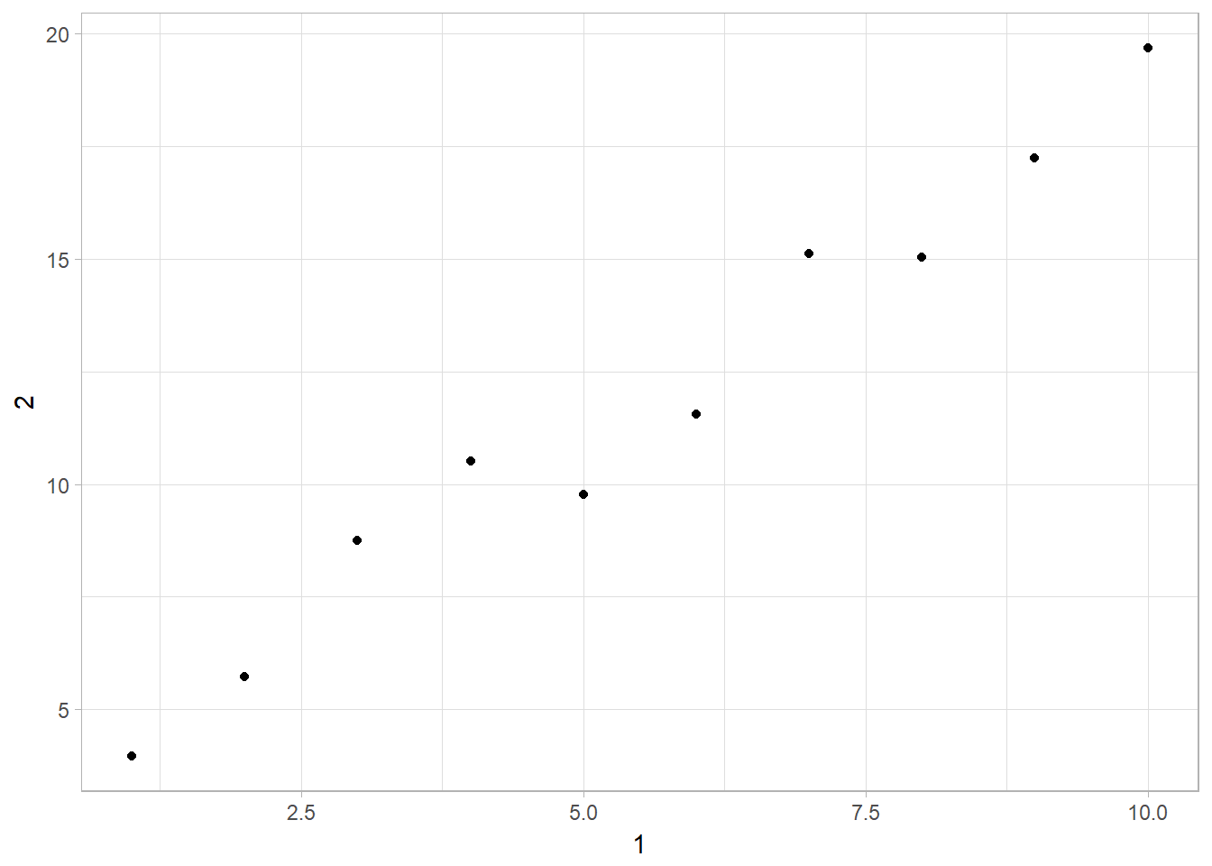
- A new column 3 which is 2 divided by 1:
annoying3 = annoying %>%
  mutate(`3` = .[["2"]]/.[["1"]])

## or an easier way: insert straight away

annoying4 = annoying
annoying4[["3"]] = annoying4[["2"]]/ annoying4[["1"]]
annoying4
## # A tibble: 10 x 3
## `1` `2` `3`
## <int> <dbl> <dbl>
## 1 1 3.97 3.97
## 2 2 5.72 2.86
## 3 3 8.75 2.92
## 4 4 10.5 2.63
## 5 5 9.77 1.95
## 6 6 11.6 1.93
## 7 7 15.1 2.16
## 8 8 15.0 1.88
## 9 9 17.3 1.92
## 10 10 19.7 1.97## or
annoying5 = annoying
annoying5$`3`= annoying4[["2"]]/ annoying4[["1"]]
annoying5## # A tibble: 10 x 3
## `1` `2` `3`
## <int> <dbl> <dbl>
## 1 1 3.97 3.97
## 2 2 5.72 2.86
## 3 3 8.75 2.92
## 4 4 10.5 2.63
## 5 5 9.77 1.95
## 6 6 11.6 1.93
## 7 7 15.1 2.16
## 8 8 15.0 1.88
## 9 9 17.3 1.92
## 10 10 19.7 1.97Check if an object is a tibble using class()
mtcars is a data.frame object:
class(mtcars)## [1] "data.frame"A tibble object would only show 10 rows and show the type of data in each column. In addition, class(mtcars) shows that it is a dataframe. Additionally, tibbles have class "tbl_df" and "tbl" in addition to "data.frame":
class(as.tibble(mtcars))## [1] "tbl_df" "tbl" "data.frame"Interacting with Older Code
Turn a tibble into dataframe using as.data.frame()
Some older functions don’t work with tibbles due to the [ function. [ is not used because dplyr::filter() and dplyr::select() allow you to solve the same problems with clearer code. If you encounter one of these functions, use as.data.frame() to turn a tibble back to a data.frame:
class(as.data.frame(tb))## [1] "data.frame"Frustrations caused by subsetting default data.frame
Let’s define a df dataframe and perform subsetting operations on it.
df <- data.frame(abc = 1, xyz = "a")
df$x
## [1] a
## Levels: adf[, "xyz"]## [1] a
## Levels: adf[, c("abc", "xyz")]## abc xyz
## 1 1 aFirst of all, dataframe partially complete a column name such that df$x is the same as df$xyz, posing the possible disaster of calling unintended variables.
Secondly, the [ object returns a vector when there is one colomn but it returns a dataframe if more than one (tibble always return tibbles). These is problematic if you are passing df[, vars], where the number of variables is unknown. You’d have to write codes to account those situations.
Let’s compare the similar code but using a tibble instead:
tb = as.tibble(df)
tb$x
## NULLtb[, "xyz"]## # A tibble: 1 x 1
## xyz
## <fct>
## 1 atb[, c("abc", "xyz")]## # A tibble: 1 x 2
## abc xyz
## <dbl> <fct>
## 1 1. a