Introduction
The K-nearest neighbors (KNN) classifier works by indentifying \(K\) (a positive integer) training data points that are closest (defined by Euclidean distance) to a test observation \(x_0\) and calculate the conditional probability of \(x_0\) belongs to class \(j\). The conditional probability equals to the fraction of the \(K\) training data points that belongs to class \(j\).
Self-defined KNN Classifier
The fields library is used here mainly for rdist(). It calculates pairwise distance between the training data points and the testing observation.
The following are the steps to create KNN classifier:
- Create inputs for \(K\), testing data, training data, and its corresponding classes.
- Calculate the distance between each training data with each testing observation. Save that in a matrix or data frame.
- For each test observation, choose the top \(k\) closest training data points to it. Set the most occuring/ common classes among the \(k\) data points as the predicted class.
It’s pretty simple, isn’t it?
Let’s work on it now.
myknn <- function(train, test, trainclass, k)
{
  # Loading library
  require(fields)
  # create an empty placeholder for predicted values
  pred = c()

  # calculate distance
  # The output of the "dist" dataframe is such that the rows are the
  #     training data points, while the columns are the testing observations.
  #     The cells for each row-column pair are the Euclidean distance from
  #     training data to the corresponsing testing data
  dist = rdist(train, test)

  # Create a loop for each testing observation
  for (i in 1:nrow(test))
  {
  nb = data.frame(dist = dist[,i], class = trainclass)

  # Ranking the rows in the dataframe by the distance from the testing
  #   observation. nb stands Neighbourhood
  nb = nb[order(nb$dist),]

  # Choose the K closest Neighbour
  topnb = nb[1:k,]

  #Deciding the Class by picking the highest occurence name.
  ans = names(sort(summary(topnb$class), decreasing=T)[1])

  # concatenate the latest prediction to the previous one
  pred = c(pred, ans)
  }
  return(pred)
}
Simulation, errors and KNN Boundary
Simulate data
Lets generate some data in two dimensions, and make them a little separated.
set.seed(101); n = 500
x = matrix(rnorm(n, sd = 5),n/2,2)
class = rep(c(1,2),each = n/4)
x[class == 1,] = x[class == 1,] + 7
plot(x,col = c("orangered", "navyblue")[class],pch = 20, xlab = "x1", ylab = "x2")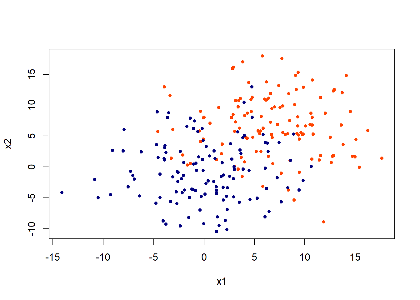
Training and Testing Errors
First, let’s split the dataset into training and testing data.
set.seed(101)
train = sample(1:n/2, n/4); test = -train
x.train = x[train,]; x.test = x[test,]
class.train = class[train]; class.test = class[test]
Perform KNN using K = 3 and 5. The choice of \(k\) is usually determine by using cross-validation but they were chosen arbitarily here.
kchoice = c(3,5)
# To store the error rate
err = matrix(NA, 2,2)
colnames(err) = c("train", "test")
rownames(err) = c("k = 3", "k = 5")

# initializa column value
j = 1

for(i in kchoice)
{
  # For training error
  pred = myknn(x.train, x.train, as.factor(class.train),k = i)
  err[j,1] = mean(pred!=as.factor(class.train))
  # For testing error
  pred = myknn(x.train, x.test, as.factor(class.train),k = i)
  err[j,2] = mean(pred!=as.factor(class.test))
  #Update
  j = j + 1
}
Let’s look at the errors.
err## train test
## k = 3 0.104 0.1726619
## k = 5 0.128 0.2086331The testing error rate is always larger than that or training error rate. In addition, using a small \(k\), such as 1, will have lower training error. In fact, using \(k =1\) will give 0 training error. We also observe that using \(k = 3\) perform better than \(k = 5\) in the test data.
Decision boundaries
Let’s define another function named as make.grid(). It is meant to expand the grid for all the x1 and x2.
make.grid=function(x,n=200){
  grange=apply(x,2,range)
  x1=seq(from=grange[1,1],to=grange[2,1],length=n)
  x2=seq(from=grange[1,2],to=grange[2,2],length=n)
  expand.grid(X1=x1,X2=x2)
}
Then, draw the decision boundary. The xgrid are the “test data” in this case but they are meant to show the decision boundary here.
First, look at KNN = 3.
xgrid = make.grid(x, n = 150)
ygrid = myknn(x,xgrid, as.factor(class), k = 3)
plot(xgrid,col=c("orange","dodgerblue")[as.numeric(ygrid)],pch = 20,cex = .2, main = "KNN = 3")
points(x,col = c("orangered", "navyblue")[class],pch = 20)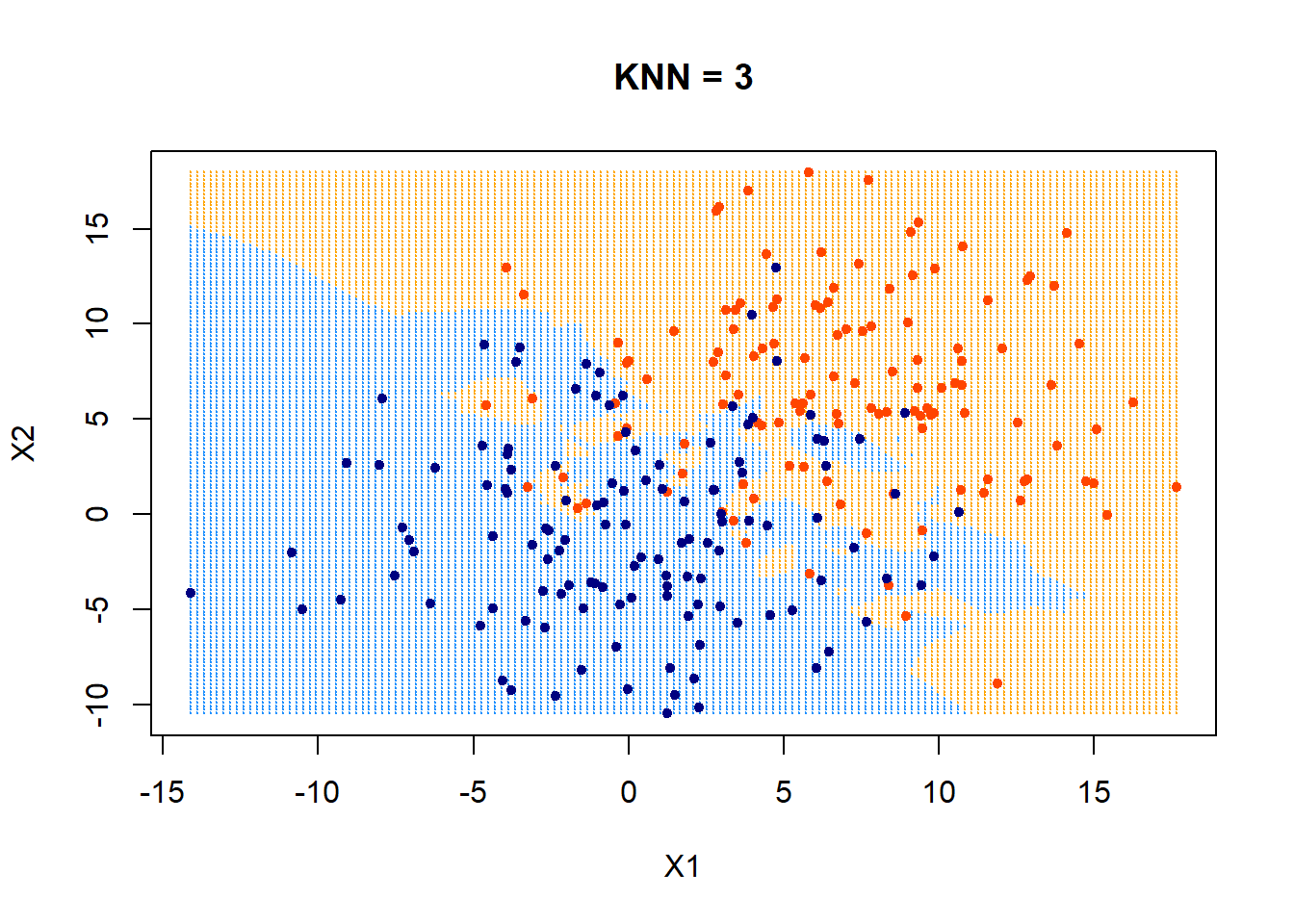
Those data points that fall outside of their boundaries (defined by colors in the plot) are classfied as errors.
The following uses KNN = 5.
ygrid = myknn(x,xgrid, as.factor(class), k = 5)
plot(xgrid,col=c("orange","dodgerblue")[as.numeric(ygrid)],pch = 20,cex = .2, main = "KNN = 5")
points(x,col = c("orangered", "navyblue")[class],pch = 20)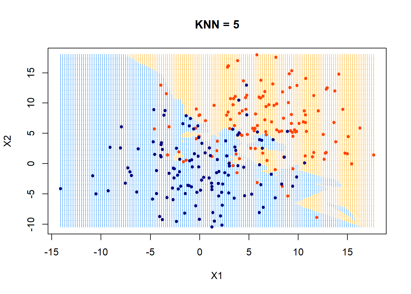
How about using KNN = 10? What would the decision boundary look like?
ygrid = myknn(x,xgrid, as.factor(class), k = 10)
plot(xgrid,col=c("orange","dodgerblue")[as.numeric(ygrid)],pch = 20,cex = .2, main = "KNN = 10")
points(x,col = c("orangered", "navyblue")[class],pch = 20)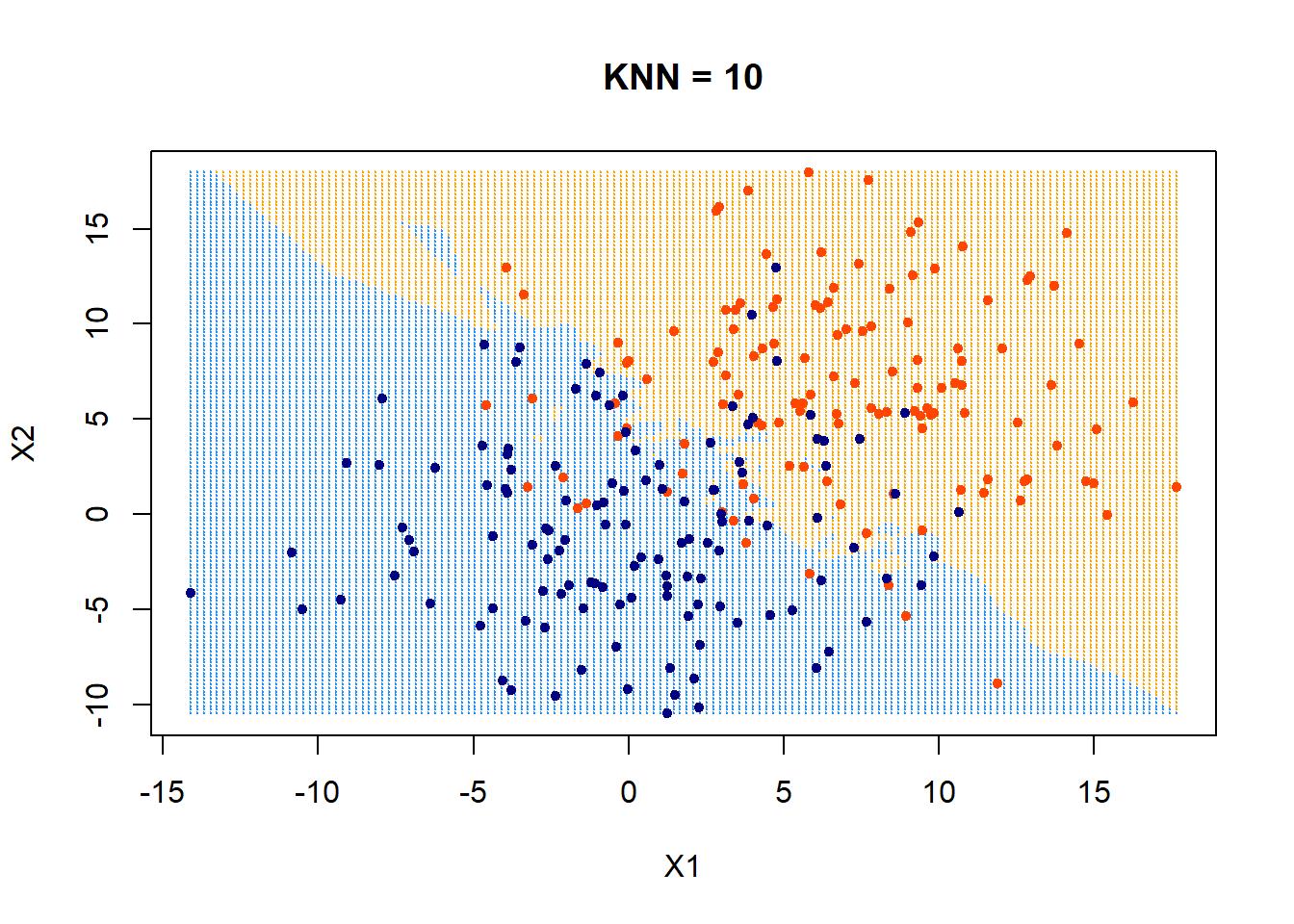 It appears that the boundary is getting more linear and less flexible now.
Next steps
The next steps after creating a KNN classifier is to generalize it to predict numerical values in addition to classes. Incorporate cross-validation options into it is also very useful.