Cross Validation Function for Classifier

Mon, Apr 16, 2018 9 min read R

Introduction

As mentioned in the previous post, the natural step after creating a KNN classifier is to define another function that can be used for cross-validation (CV).

The kind of CV function that will be created here is only for classifier with one tuning parameter. This includes the KNN classsifier, which only tunes on the parameter $K$.

Self-defined functions

`cvclassifier`

Arguments and Values

cvclassifier has the following parameters:

data: These are the training data
class: These are classes (or groups) for the training data
classifier: The type of classifier (i.e., KNN classifier)
fold: Number of folds used in cross validation. The default value is 10.
seed: Seed number for partitioning data into folds. The default value is 1001.
… : Any arguments to be passed to the classifier

Note that it is assumed that the classifier has the arguments in the following order: classifier(traindat, testdat, trainclass, …)

cvclassifier returns the following:

cverror: The cross-validation error for the specified number of folds and tuning parameter value.
trainpred: The predicted classes for the training data for the specified tuning parameter value.

Implementations

The steps of implementing cvclassifier:

Make sure that the number of folds is smaller than number of observations. Abort if that is not satisfied.
Set a seed value and shuffle the rows of the dataset (means the data and class) before partitioning into m folds. Make sure to keep a copy of the original dataset for future use.
Assign indexes showing which fold that each row belongs to. Try to make the number of observation in each group to be the same. If not possible, randomly assign the remaining observation into any folds.
For $i = 1,..., m$, use the $ith$ fold as the testing data and the $m-1$ folds as the training data. With a specified tuning parameter value, use the classifier to predict the classes of testing data and record the rate of misclassification. Repeat this step for $m$ times.
Return the average error rate and the predicted classes using the whole training data.

cvclassifier <-  function(data, class, classifier, fold = 10, seed = 1001, ...)
{
  # Condition check first
  if (nrow(data) < fold) try(stop("Number of folds is greater than number of observations.\n Reduce numder of folds."))
  
  # Set a random seed to control for results
  set.seed(seed)
  # Make a copy of original dataand class
  oridata = data
  oriclass = class
  # Shuffle data and break into k folds
  shuffle_index <- sample.int(nrow(data))
  data <- data[shuffle_index, ]
  class <- class[shuffle_index]
  
  # Partition data (into m folds)
  num_per_fold <- nrow(data) %/% fold
  remaining <- nrow(data) %% fold
  # Initialize space holder that deffines which fold each observation belongs to
  part_data <- c()
  # Allocating folds
  for (j in 1:fold)
  {
    part_data <- c(part_data, rep(j, num_per_fold))
  }
  # Fill in the remaining randomly into any fold
  if(remaining != 0){
    for (k in 1:remaining)
    {
      part_data <- c(part_data, rep(sample.int(fold,1), 1))
    }
  }
  # For each fold, use the classsifer to fit and calculate testing error
  # Initialize error rate
  err <- 0
  for (i in 1 : fold)
  {
    test_index = which(part_data == i, arr.ind = TRUE)
    train_index <-  -test_index
    testdat <- data[test_index,]; testclass = class[test_index]
    traindat <- data[train_index,]; trainclass = class[train_index]
    
    ## Use classifier
    pred <- classifier(traindat, testdat, trainclass, ...)
    err <- err + mean(pred != testclass)
  }
  
  # The avearge of error
   err <- err/fold
  
  # Predicted values of all data
   pred_train <- classifier(oridata, oridata, oriclass, ...)

  # Return the results
  return(list(cverror = err, trainpred = pred_train))
}

The function defined here is good enough to perform cross validation with a specified tuning parameter value. Let’s define another function that allows us to try on a range of tuning parameter values before choosing the best one.

`classpred.cv`

Arguments and Values

classpred.cv has the following parameters:

traindat: The training dataset
trainclass: The training data’s classes
testdat: The testing dataset.
testclass: The testing data’s classes
classifier: Type of classifier to be used such as KNN classifier.
parameter: Tuning parameter values. It is usually entered as a vector. The default value is NULL.
fold: $m$ fold for CV purpose. The default value is 10.
seed: Seed value. The default value is 1001.

classpred.cv returns the following:

train_pred: Predicted classes for training data.
train_err: Training data error rate.
test_pred: Predicted classes for testing data. The prediction is done based on the parameter value that gives the lowest cross-validated error.
test_err: Testing data error rate.
parameter: Values of parameter used.
best_param: The best tuning parameter. It’s the parameter value that gives the lowest CV error.
cverror: Cross-validated errors in training data for all parameter values.
cvpred: Predicted classes for training data for all parameter values.
plot: Allow user to plot cverror vs parameter.

Implementations

The steps of implementing classpred.cv:

Make sure that at least a tuning parameter value is provided. Abort if no value was provided.
For each of the parameter values, collect the cross-validated error and train data predicted classes from the cvclassifier.
Save the best training data predicted classes. The predicted classes are chosen by using the tuning parameter value that minimizes the cross-validation error, $tune_{best}$. Calculate the training error too.
Predict the classses for testing data using $tune_{best}$ and calculate the testing error.
Using ggplot2 to create and save a plot object.

classpred.cv <- function(traindat, trainclass, testdat, testclass,
                         classifier, parameter=NULL, fold = 10, seed = 1001)
{
  if (is.null(parameter)) try(stop ("No parameter range stated"))
  
  trainclass <- as.factor(trainclass)
  # prediction list
  cvpred <- list()
  ## error list
  cverror <- c()
  
  for (i in parameter)
  {
    results <- cvclassifier(traindat, trainclass, classifier,
                            fold, seed, i)
    cvpred [[i]] <- results$trainpred
    cverror <- c(cverror, results$cverror)
  }
  
  #Clearing up the NULL elements
  cvpred[sapply(cvpred,is.null)] <- NULL

  train_pred = cvpred [[which.min(cverror)]]
  train_err <- mean(train_pred!=trainclass)
  
  #Predict using the best parameter
  test_pred = classifier(traindat, testdat, 
                         trainclass, parameter[which.min(cverror)])
  
  # calculated test error
  test_err = mean(test_pred!=testclass)
  
  
  cat("The best parameter is ", parameter[which.min(cverror)], 
      "with cross-validated error of ", cverror[which.min(cverror)], ".\n")
  cat("The training error using parameter = ", parameter[which.min(cverror)], 
      " is ", train_err, ". \n")
  cat("The testing error using parameter = ", parameter[which.min(cverror)], 
      " is ", test_err, ".")
  
  require(ggplot2)
  p.plot <- qplot(data =as.data.frame(cbind(parameter,cverror)),
                  x = parameter,
                  y = cverror,
                  geom = c("point", "line"),
                  main = "Cross Validation Error across parameter values",
                  xlab = "Values of parameter",
                  ylab = "C.V. Error",
                  colour = I("dodgerblue"),
                  size = I(1))
  
  return(list(train_pred=train_pred, 
         train_err = train_err,
         test_pred = test_pred,
         test_err = test_err,
         parameter = parameter,
         best_param = parameter[which.min(cverror)],
         cverror = cverror,
         cvpred =  cvpred,
         plot = p.plot))
}

Simulation, Errors and KNN Boundaries

Example 1

Simulate Data

Lets generate some data in two dimensions. Three classes (groups) are created.

set.seed(1001); n = 600
x = matrix(rnorm(n, sd = 4),n/2,2)
class = rep(c(1,2,3),each = n/6)
x[class == 1,] = x[class == 1,] + 7
x[class == 2,] = x[class == 2,] + 12
x[class == 2,2] = x[class == 2,2] - 15
plot(x,col = c("orangered", "navyblue", "green3")[class],pch = 20, xlab = "x1", ylab = "x2")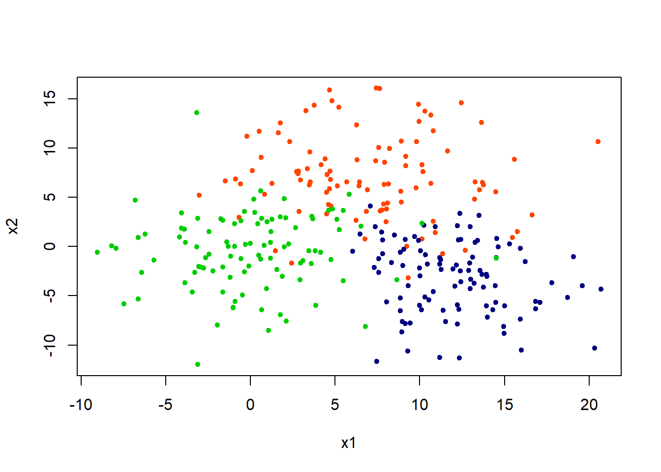

Training and Testing Errors

First, let’s split the dataset into training and testing data.

set.seed(1001)
train = sample.int(n/2, n/4); test = -train
x.train = x[train,]; x.test = x[test,]
class.train = class[train]; class.test = class[test]

Cross Validation

Let’s use the classpred.cv function to choose the best number of $K$ depending on the cross-validated error. Let’s use 10 folds in this case and set the tuning parameter values range from 1 to 100.

pred = classpred.cv(x.train, as.factor(class.train), x.test, class.test,
                    myknn, parameter = 1:100, fold = 10, seed = 1001)

## The best parameter is  17 with cross-validated error of  0.1066667 .
## The training error using parameter =  17  is  0.1066667 . 
## The testing error using parameter =  17  is  0.1066667 .

We can even plot the cross validation error as a function of tuning parameter using pred$plot

pred$plot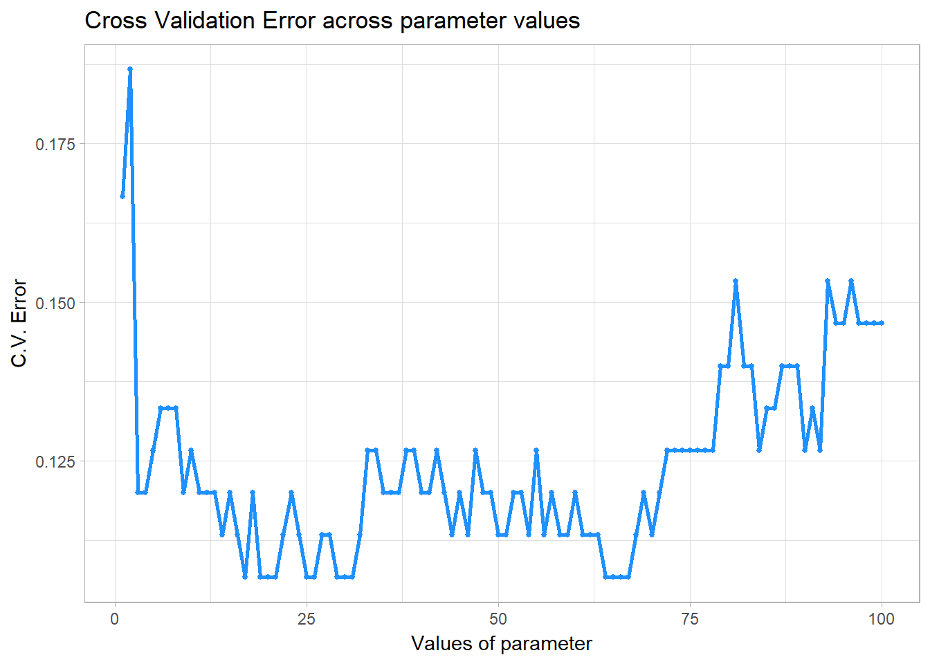

Decision Boundaries

Let’s visualise the decision boundary with three separate groups. We will be using the make.grid function defined in the [previous post] (https://theanlim.rbind.io/post/k-nearest-neighbour-classifier-self-written-function/).

xgrid = make.grid(x, n = 150)
ygrid = myknn(x,xgrid, class, k = pred$best_param)
plot(xgrid,col=c("orange","dodgerblue","palegreen3")[as.numeric(ygrid)],pch = 20,cex = .2, main = paste("K = ", pred$best_param))
points(x,col = c("orangered", "navyblue", "green3")[class],pch = 20)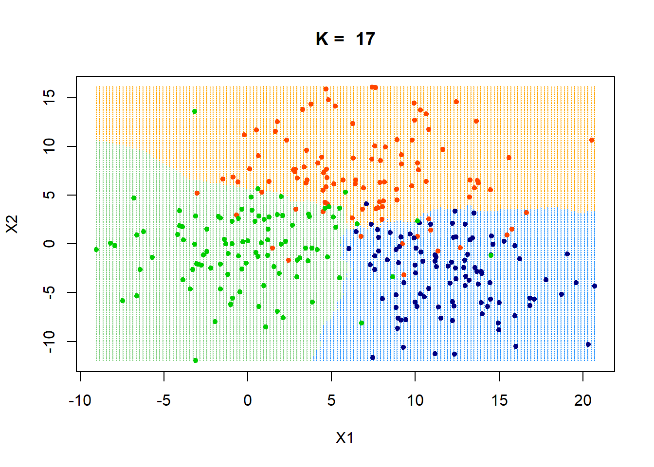

Example 2

Let’s try working on another example. We will start with simulating the data first. This data is simulated such that the overlap between classes is minimal.

Simulate Data

set.seed(1001)
r1 = runif(n/3, -1,1)
r2 = c(runif(n/6,-2,-1), runif(n/6,1,2))
r3 = -r2
rad = seq(1,2*pi, length = n/3)
x1 <- c(r1*cos(rad), r2*cos(rad), r3*cos(rad) )
x2 <- c(r1*sin(rad), r2*sin(rad), r3*sin(rad))
x = cbind(x1,x2)
class = rep(c(1,2, 3), each=n/3 )
plot(x1, x2 , col = c("orangered", "navyblue", "green3")[class], pch = 20)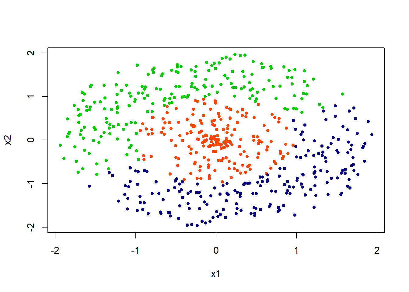

The aim in this example in to explore whether KNN classifier is able to distiguish classes that are nested (i.e., the orange dots are surrounded by two different classes)

Training and Testing Errors

First, let’s split the dataset into training and testing data.

set.seed(1001)
train = sample.int(n, n/2)
test = -train
x.train = x[train,]
x.test = x[test,]
class.train = class[train]; class.test = class[test]

Cross Validation

Again, let’s use 10 folds in this case and set the tuning parameter values range from 1 to 100.

pred = classpred.cv(x.train, as.factor(class.train), x.test, class.test,
                    myknn, parameter = 1:100, fold = 10, seed = 1001)

## The best parameter is  5 with cross-validated error of  0.04333333 .
## The training error using parameter =  5  is  0.03 . 
## The testing error using parameter =  5  is  0.04 .

Plot the cross validation error as a function of tuning parameter using pred$plot

pred$plot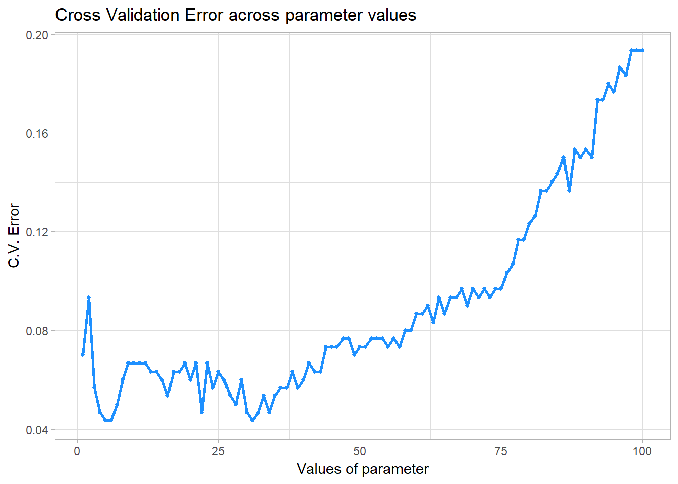

The plot shows that a lower value of $K$ performs better as it has a lower cross validation error. This makes sense because, by definition, increasing the number of $k$ expands its neighbourhood in a circular way and that is only helpful to the orange points on the plot, but not the others. The other two groups form curvature shapes on the X1 - X2 dimension.

In addition, a small $k$ is all we need because the classes are highly separable. We see a lower test error in this example compared to Example 1 because the classes are separated pretty cleanly.

Decision Boundaries

How would the decision boundaries look like?

xgrid = make.grid(x, n = 150)
ygrid = myknn(x,xgrid, class, k = pred$best_param)
plot(xgrid,col=c("orange","dodgerblue","palegreen3")[as.numeric(ygrid)],pch = 20,cex = .2, main = paste("K = ", pred$best_param))
points(x,col = c("orangered", "navyblue", "green3")[class],pch = 20)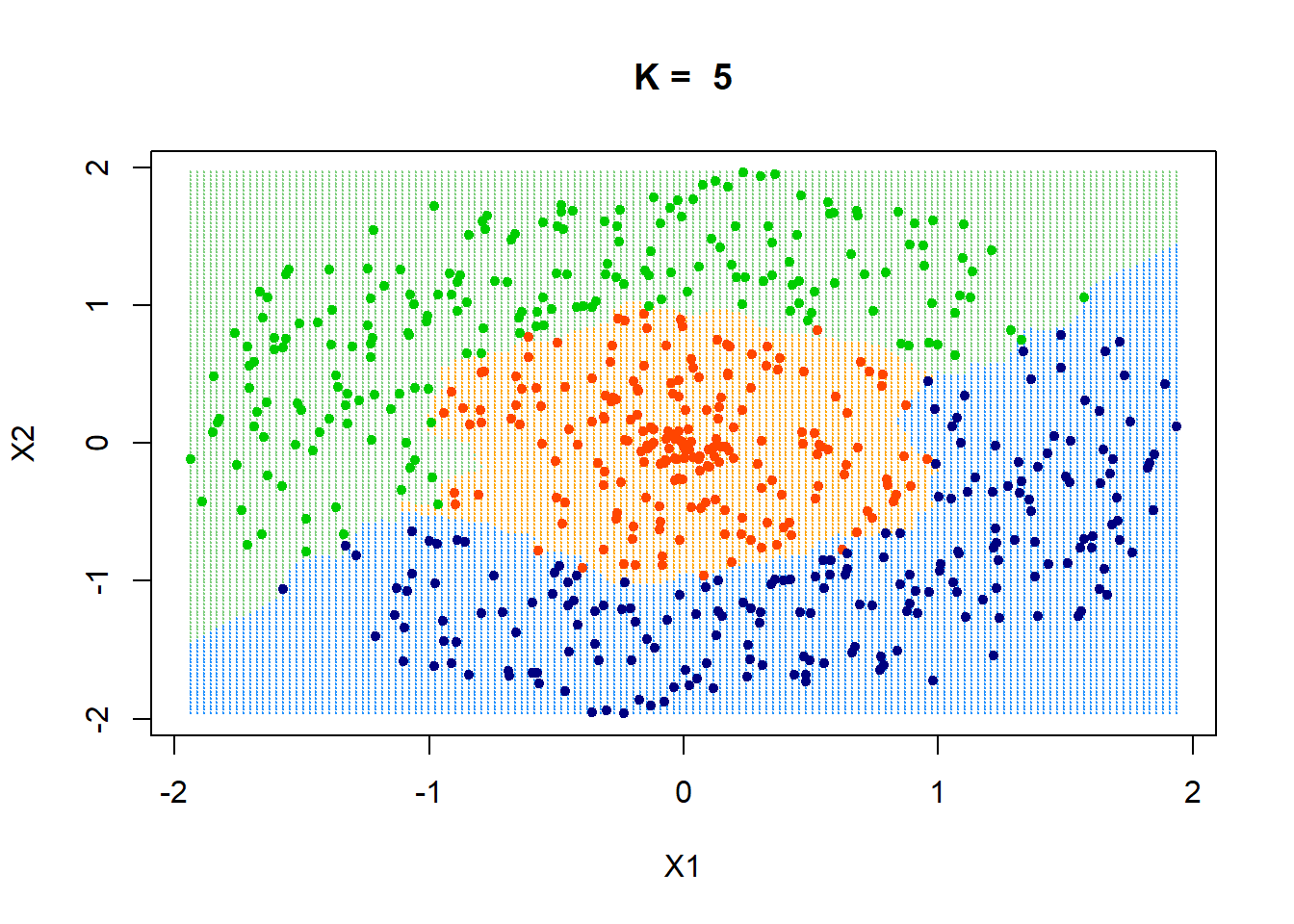

It seems like the decision boundaries are flexible enough to classify correctly.

Next Steps

We have finally created KNN classifier and a cross-validated function for classifiers. One can explore and create other classifiers in addition to KNN classifier. Besides, the KNN classfier is also applicable in higher dimensions space. How would the visualization of 3D decision boundaries would look like?

classification function machine-learning simulation

Cross Validation Function for Classifier

Introduction

Self-defined functions

cvclassifier

Arguments and Values

Implementations

classpred.cv

Arguments and Values

Implementations

Simulation, Errors and KNN Boundaries

Example 1

Simulate Data

Training and Testing Errors

Cross Validation

Decision Boundaries

Example 2

Simulate Data

Training and Testing Errors

Cross Validation

Decision Boundaries

Next Steps

Related

`cvclassifier`

`classpred.cv`