Tidy Data with tidyr

Thu, Jul 12, 2018 23 min read R

Tidy Data
Spreading and Gathering
Separating and Uniting
Missing Values
Comparing the fill arguments of spread() and complete()
Nontidy Data

** This post is heavily based on R for Data Science. Please consider to buy that book if you find this post useful.**

tidyr, a member of the core tidyverse, will be used in this chapter.

Tidy Data

The tidy dataset, will be much easier to work with inside the tidyverse.
There are three interrelated rules which make a dataset tidy:

Each variable must have its own column.
Each observation must have its own row.
Each value must have its own cell.

That interrelationship leads to an even simpler set of practical instructions:

Put each dataset in a tibble.
Put each variable in a column.

The two main advantages of tidy data:

Due to having a consistent data structure (i.e., tidy data), it’s easier to learn the tools that work with it because they have an underlying uniformity.
There’s a specific advantage to placing variables in columns because it allows R’s vectorized nature to shine. Most built-in R functions work with vectors of values. That makes transforming tidy data feel particularly natural.

All of the packages in the tidyverse are designed to work with tidy data. For example:

# Compute rate per 10,000
table1 %>%
  mutate(rate = cases / population * 10000)

## # A tibble: 6 x 5
##   country      year  cases population  rate
##   <chr>       <int>  <int>      <int> <dbl>
## 1 Afghanistan  1999    745   19987071 0.373
## 2 Afghanistan  2000   2666   20595360 1.29 
## 3 Brazil       1999  37737  172006362 2.19 
## 4 Brazil       2000  80488  174504898 4.61 
## 5 China        1999 212258 1272915272 1.67 
## 6 China        2000 213766 1280428583 1.67

# Compute cases per year
table1 %>%
  count(year, wt = cases)

## # A tibble: 2 x 2
##    year      n
##   <int>  <int>
## 1  1999 250740
## 2  2000 296920

# Visualize changes over time
library(ggplot2)
ggplot(table1, aes(year, cases)) +
  geom_line(aes(group = country), color = "grey50") +
  geom_point(aes(color = country))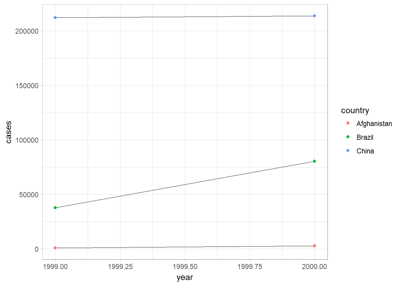

Spreading and Gathering

Most data that you will encounter will be untidy. There are two main reasons:

Most people aren’t familiar with the principles of tidy data, and it’s hard to derive them yourself unless you spend a lot of time working with data.
Data is often organized to facilitate some use other than analysis. For example, data is often organized to make entry as easy as possible.

Thus, you need to do some tidying for the most of the datasets:

Figure out what the variables and observations are.
Resolve one of two common problems using tidyr’s gather() and spread():
1. One variable might be spread across multiple columns. Use gather() for this.
2. One observation might be scattered across multiple rows. Use spread() for this.

Gathering by `gather(data, key, value, cols_selection)`

A common problem is a dataset where some of the column names are not names of variables, but values of a variable.

For example, column names 1999 and 2000 represent values of the year variable in table4a,and each row represents two observations, not one:

table4a

## # A tibble: 3 x 3
##   country     `1999` `2000`
## * <chr>        <int>  <int>
## 1 Afghanistan    745   2666
## 2 Brazil       37737  80488
## 3 China       212258 213766

To tidy a dataset like this, we need to gather those columns into a new pair of variables.

gather(data, value_column, key_var_name, spreading_value)

The set of columns that represent values, not variables. In this example, those are the columns 1999 and 2000.
The name of the variable whose values form the column names. I call that the key, and here it is year.
The name of the variable whose values are spread over the cells. I call that value, and here it’s the number of cases.

table4a %>%
`gather(`1999`, `2000`, key = "year", value = "cases")

table4b %>%
  gather(`1999`, `2000`, key = "year", value = "population")

## Error: <text>:2:10: unexpected numeric constant
## 1: table4a %>%
## 2: `gather(`1999
##             ^

To combine the tidied versions of table4a and table4b into a single tibble, we need to use dplyr::left_join():

tidy4a <- table4a %>%
  gather(`1999`, `2000`, key = "year", value = "cases")
tidy4b <- table4b %>%
  gather(`1999`, `2000`, key = "year", value = "population")
left_join(tidy4a, tidy4b)

## # A tibble: 6 x 4
##   country     year   cases population
##   <chr>       <chr>  <int>      <int>
## 1 Afghanistan 1999     745   19987071
## 2 Brazil      1999   37737  172006362
## 3 China       1999  212258 1272915272
## 4 Afghanistan 2000    2666   20595360
## 5 Brazil      2000   80488  174504898
## 6 China       2000  213766 1280428583

Spreading with `spread(data, key, value, fill = NA)`

Spreading is the opposite of gathering. You use it when an observation is scattered across multiple rows. Thus, spread and gather are complement.

For example, take table2-an observation is a country in a year, but each observation is spread across two rows:

table2

## # A tibble: 12 x 4
##    country      year type            count
##    <chr>       <int> <chr>           <int>
##  1 Afghanistan  1999 cases             745
##  2 Afghanistan  1999 population   19987071
##  3 Afghanistan  2000 cases            2666
##  4 Afghanistan  2000 population   20595360
##  5 Brazil       1999 cases           37737
##  6 Brazil       1999 population  172006362
##  7 Brazil       2000 cases           80488
##  8 Brazil       2000 population  174504898
##  9 China        1999 cases          212258
## 10 China        1999 population 1272915272
## 11 China        2000 cases          213766
## 12 China        2000 population 1280428583

The syntax of spread is:

spread(dataframe, key = col_name_or_position_of_var, value = cols_with_multiple_vars_values, fill = NA)

spread(table2, key = type, value = count)

## # A tibble: 6 x 4
##   country      year  cases population
##   <chr>       <int>  <int>      <int>
## 1 Afghanistan  1999    745   19987071
## 2 Afghanistan  2000   2666   20595360
## 3 Brazil       1999  37737  172006362
## 4 Brazil       2000  80488  174504898
## 5 China        1999 212258 1272915272
## 6 China        2000 213766 1280428583

fill = ensures that missing values will be replaced by this value.

spread() and gather() are complements. gather() makes wide tables narrower and longer; spread() makes long tables shorter and wider.

Unique identifiers in `spread`

Spreading this tibble would fail:

people <- tribble(
  ~name,             ~key,    ~value,
  #-----------------|--------|------
  "Phillip Woods",   "age",       45,
  "Phillip Woods",   "height",   186,
  "Phillip Woods",   "age",       50,
  "Jessica Cordero", "age",       37,
  "Jessica Cordero", "height",   156
)
spread(people, key, value)

## Error: Duplicate identifiers for rows (1, 3)

Spreading the tibble fails because there are two rows with “age” for “Phillip Woods”. We would need to add another column with an indicator for the number observation it is:

people[["id"]] <- c(1,1,2,3,3)
spread(people, key, value)

## # A tibble: 3 x 4
##   name               id   age height
##   <chr>           <dbl> <dbl>  <dbl>
## 1 Jessica Cordero    3.   37.   156.
## 2 Phillip Woods      1.   45.   186.
## 3 Phillip Woods      2.   50.    NA

Imperfect symmetrical complement of `spread` and `gather`| unless `convert = TRUE`

For example:

stocks <- tibble(
  year   = c(2015, 2015, 2016, 2016),
  half  = c(   1,    2,     1,    2),
  return = c(1.88, 0.59, 0.92, 0.17)
)
stocks %>%
  spread(year, return) %>%
  gather("year", "return", `2015`:`2016`)

## # A tibble: 4 x 3
##    half year  return
##   <dbl> <chr>  <dbl>
## 1    1. 2015   1.88 
## 2    2. 2015   0.590
## 3    1. 2016   0.920
## 4    2. 2016   0.170

The functions spread and gather are not perfectly symmetrical because column type information is not transferred between them. In the original table the column year was numeric, but after running spread() and gather() it is a character vector. This is because the key variable names are always converted to a character vector by gather() or it will be saved as factor if the factor_key = TRUE.

The convert argument tries to convert character vectors to the appropriate type. In the background this uses the type.convert function.

stocks %>%
  spread(year, return) %>%
  gather("year", "return", `2015`:`2016`, convert = TRUE)

## # A tibble: 4 x 3
##    half  year return
##   <dbl> <int>  <dbl>
## 1    1.  2015  1.88 
## 2    2.  2015  0.590
## 3    1.  2016  0.920
## 4    2.  2016  0.170

Separating and Uniting

Separate by `separate(data, ... = col_to_be_separated, into = new_vars_name)`

separate() pulls apart one column into multiple columns, by splitting wherever a separator character appears.

The rate column in table3 contains both cases and population variables and we need to split it into two variables.

separate(data, col_to_be_separated, into = new_vars_name)

table3 %>%
  separate(rate, into = c("cases", "population"))

## # A tibble: 6 x 4
##   country      year cases  population
## * <chr>       <int> <chr>  <chr>     
## 1 Afghanistan  1999 745    19987071  
## 2 Afghanistan  2000 2666   20595360  
## 3 Brazil       1999 37737  172006362 
## 4 Brazil       2000 80488  174504898 
## 5 China        1999 212258 1272915272
## 6 China        2000 213766 1280428583

Type conversion by `convert = TRUE`

Note that the default behavior in separate(): it leaves the type of the column as it originally is. However, We can ask separate() to try and convert to better types using convert = TRUE:

table3 %>%
  separate(
    rate,
    into = c("cases", "population"),
    convert = TRUE
  )

## # A tibble: 6 x 4
##   country      year  cases population
## * <chr>       <int>  <int>      <int>
## 1 Afghanistan  1999    745   19987071
## 2 Afghanistan  2000   2666   20595360
## 3 Brazil       1999  37737  172006362
## 4 Brazil       2000  80488  174504898
## 5 China        1999 212258 1272915272
## 6 China        2000 213766 1280428583

Specific character as split values by `sep = "/"`

By default, separate() will split values wherever it sees a nonalphanumeric character (i.e., a character that isn’t a number or letter). If you wish to use a specific character to separate a column, you can pass the character to the sep argument of separate().

table3 %>%
  separate(rate, into = c("cases", "population"), sep = "/")

## # A tibble: 6 x 4
##   country      year cases  population
## * <chr>       <int> <chr>  <chr>     
## 1 Afghanistan  1999 745    19987071  
## 2 Afghanistan  2000 2666   20595360  
## 3 Brazil       1999 37737  172006362 
## 4 Brazil       2000 80488  174504898 
## 5 China        1999 212258 1272915272
## 6 China        2000 213766 1280428583

(Formally, sep is a regular expression)

Split by vector of integers by `sep = c(2,4)`

You can also pass a vector of integers to sep. separate() will interpret the integers as positions to split at:

Positive values start at 1 on the far left of the strings;
negative values start at -1 on the far right of the strings.

When using integers to separate strings, the length of sep should be one less than the number of names in into. For example,

table3 %>%
  separate(year, into = c("century", "decade", "year"), sep = c(2,3))

## # A tibble: 6 x 5
##   country     century decade year  rate             
## * <chr>       <chr>   <chr>  <chr> <chr>            
## 1 Afghanistan 19      9      9     745/19987071     
## 2 Afghanistan 20      0      0     2666/20595360    
## 3 Brazil      19      9      9     37737/172006362  
## 4 Brazil      20      0      0     80488/174504898  
## 5 China       19      9      9     212258/1272915272
## 6 China       20      0      0     213766/1280428583

`extra` in `separate`

The extra argument tells separate what to do if there are too many pieces.

For example:

tibble(x = c("a,b,c", "d,e,f,g", "h,i,j"))

## # A tibble: 3 x 1
##   x      
##   <chr>  
## 1 a,b,c  
## 2 d,e,f,g
## 3 h,i,j

We can see that we have an extra g.

By default separate drops the extra values with a warning:

tibble(x = c("a,b,c", "d,e,f,g", "h,i,j")) %>%
  separate(x, c("one", "two", "three"))

## # A tibble: 3 x 3
##   one   two   three
##   <chr> <chr> <chr>
## 1 a     b     c    
## 2 d     e     f    
## 3 h     i     j

The following produces the same result as above, dropping extra values, but without the warning:

tibble(x = c("a,b,c", "d,e,f,g", "h,i,j")) %>%
  separate(x, c("one", "two", "three"), extra = "drop")

## # A tibble: 3 x 3
##   one   two   three
##   <chr> <chr> <chr>
## 1 a     b     c    
## 2 d     e     f    
## 3 h     i     j

In the following, the extra values are not split, so “f,g” appears in column three:

tibble(x = c("a,b,c", "d,e,f,g", "h,i,j")) %>%
  separate(x, c("one", "two", "three"), extra = "merge")

## # A tibble: 3 x 3
##   one   two   three
##   <chr> <chr> <chr>
## 1 a     b     c    
## 2 d     e     f,g  
## 3 h     i     j

`fill` in `separate`

The fill argument tells separate what to do if there aren’t enough pieces. Now, let’s look at another tibble where we don’t have enough entries (g is missing in this case):

tibble(x = c("a,b,c", "d,e", "f,g,i"))

## # A tibble: 3 x 1
##   x    
##   <chr>
## 1 a,b,c
## 2 d,e  
## 3 f,g,i

The default for fill is similar to separate; it fills with missing values but emits a warning. In this, row 2 of column “three”, is NA:

tibble(x = c("a,b,c", "d,e", "f,g,i")) %>%
  separate(x, c("one", "two", "three"))

## # A tibble: 3 x 3
##   one   two   three
##   <chr> <chr> <chr>
## 1 a     b     c    
## 2 d     e     <NA> 
## 3 f     g     i

Alternative options for fill are "right", to fill with missing values from the right, but without a warning:

tibble(x = c("a,b,c", "d,e", "f,g,i")) %>%
  separate(x, c("one", "two", "three"), fill = "right")

## # A tibble: 3 x 3
##   one   two   three
##   <chr> <chr> <chr>
## 1 a     b     c    
## 2 d     e     <NA> 
## 3 f     g     i

The option fill = "left" also fills with missing values without a warning, but this time from the left side. Now, column “one” of row 2 will be missing, and the other values in that row are shifted over:

tibble(x = c("a,b,c", "d,e", "f,g,i")) %>%
  separate(x, c("one", "two", "three"), fill = "left")

## # A tibble: 3 x 3
##   one   two   three
##   <chr> <chr> <chr>
## 1 a     b     c    
## 2 <NA>  d     e    
## 3 f     g     i

Unite with `unite(data, col = new_col_name, ... = selection_of_cols, sep = "_", remove = TRUE)`

unite() is the inverse of separate(): it combines multiple columns into a single column.

We can use unite() to rejoin the century and year columns in table5.

unite(data, col = new_col_name, ... = selection_of_cols, sep = "_", remove = TRUE)

remove If TRUE, remove input columns from output data frame.

table5 %>%
  unite(col = new, century, year, sep = "")

## # A tibble: 6 x 3
##   country     new   rate             
##   <chr>       <chr> <chr>            
## 1 Afghanistan 1999  745/19987071     
## 2 Afghanistan 2000  2666/20595360    
## 3 Brazil      1999  37737/172006362  
## 4 Brazil      2000  80488/174504898  
## 5 China       1999  212258/1272915272
## 6 China       2000  213766/1280428583

`remove` in `unite()` and `separate()`

Both unite() and separate() have a remove argument. It will remove the old variables if it is set to TRUE. You would set it to FALSE if you want to create a new variable while keeping the old one.

Missing Values

Surprisingly, a value can be missing in one of two possible ways:

Explicitly, i.e., flagged with NA.
Implicitly, i.e., simply not present in the data.

For example:

stocks <- tibble(
  year = c(2015, 2015, 2015, 2015, 2016, 2016, 2016),
  qtr = c( 1, 2, 3, 4, 2, 3, 4),
  return = c(1.88, 0.59, 0.35, NA, 0.92, 0.17, 2.66)
)

There are two missing values in this dataset:

The return for the fourth quarter of 2015 is explicitly missing, because the cell where its value should be instead contains NA.
The return for the first quarter of 2016 is implicitly missing, because it simply does not appear in the dataset.

The way that a dataset is represented can make implicit values explicit. For example, we can make the implicit missing value explicit by putting years in the columns:

stocks %>%
  spread(year, return)

## # A tibble: 4 x 3
##     qtr `2015` `2016`
##   <dbl>  <dbl>  <dbl>
## 1    1.  1.88  NA    
## 2    2.  0.590  0.920
## 3    3.  0.350  0.170
## 4    4. NA      2.66

Turning explicit to implicit missing values using `na.rm = TRUE`

Because these explicit missing values may not be important in other representations of the data, you can set na.rm = TRUE in gather() to turn explicit missing values implicit:

stocks %>%
  spread(year, return) %>%
  gather(year, return, `2015`:`2016`, na.rm = TRUE)

## # A tibble: 6 x 3
##     qtr year  return
## * <dbl> <chr>  <dbl>
## 1    1. 2015   1.88 
## 2    2. 2015   0.590
## 3    3. 2015   0.350
## 4    2. 2016   0.920
## 5    3. 2016   0.170
## 6    4. 2016   2.66

Filling in explicit NAs with `complete()`

complete() takes a set of columns, and finds all unique combinations. It then ensures the original dataset contains all those values, filling in explicit NAs where necessary:

stocks %>%
  complete(year, qtr)

## # A tibble: 8 x 3
##    year   qtr return
##   <dbl> <dbl>  <dbl>
## 1 2015.    1.  1.88 
## 2 2015.    2.  0.590
## 3 2015.    3.  0.350
## 4 2015.    4. NA    
## 5 2016.    1. NA    
## 6 2016.    2.  0.920
## 7 2016.    3.  0.170
## 8 2016.    4.  2.66

Filling in missing values from recent entries with `fill(data, column)`

When a data source has primarily been used for data entry, missing values may indicate that the previous value should be carried forward:

treatment <- tribble(
  ~ person,           ~ treatment, ~response,
  "Derrick Whitmore", 1,           7,
  NA,                 2,           10,
  NA,                 3,           9,
  "Katherine Burke",  1,           4
)

You can fill in these missing values with fill(). It takes a set of columns where you want missing values to be replaced by the most recent nonmissing value (sometimes called last observation carried forward):

treatment %>%
  fill(person)

## # A tibble: 4 x 3
##   person           treatment response
##   <chr>                <dbl>    <dbl>
## 1 Derrick Whitmore        1.       7.
## 2 Derrick Whitmore        2.      10.
## 3 Derrick Whitmore        3.       9.
## 4 Katherine Burke         1.       4.

`direction` in `fill()`

fill(data, ..., .direction = c("down", "up"))

With fill, it determines whether NA values should be replaced by the previous non-missing value ("down"), which is the default, or the next non-missing value ("up").

Comparing the `fill` arguments of `spread()` and `complete()`

`spread(data, key, value, fill = NA vs complete(data, ..., fill = list())

Both replace both explicit and implicit NA.
spread(): If the tidy structure creates combinations of variables that do not exist in the original data set, spread() will place an NA in the resulting cells. NA is R’s missing value symbol. You can change this behaviour by passing fill an alternative value to use.

complete() A named list that for each variable supplies a single value to use instead of NA for missing combinations.

For example:

df <- tibble(
              group = c(1:2, 1),
              item_id = c(1:2, 2),
              item_name = c("a", "b", "b"),
              value1 = 1:3,
              value2 = 4:6
            )

## W/O specifying the fill
df %>% complete(group, nesting(item_id, item_name))

## # A tibble: 4 x 5
##   group item_id item_name value1 value2
##   <dbl>   <dbl> <chr>      <int>  <int>
## 1    1.      1. a              1      4
## 2    1.      2. b              3      6
## 3    2.      1. a             NA     NA
## 4    2.      2. b              2      5

## Specify a list for the missing value in value1
df %>% complete(group, nesting(item_id, item_name), 
                fill = list(value1 = 0))

## # A tibble: 4 x 5
##   group item_id item_name value1 value2
##   <dbl>   <dbl> <chr>      <dbl>  <int>
## 1    1.      1. a             1.      4
## 2    1.      2. b             3.      6
## 3    2.      1. a             0.     NA
## 4    2.      2. b             2.      5

# Case study

The tidyr::who dataset contains tuberculosis (TB) cases broken down by year, country, age, gender, and diagnosis method. Let’ take a look at the dataset:

who

## # A tibble: 7,240 x 60
##    country     iso2  iso3   year new_sp_m014 new_sp_m1524 new_sp_m2534
##    <chr>       <chr> <chr> <int>       <int>        <int>        <int>
##  1 Afghanistan AF    AFG    1980          NA           NA           NA
##  2 Afghanistan AF    AFG    1981          NA           NA           NA
##  3 Afghanistan AF    AFG    1982          NA           NA           NA
##  4 Afghanistan AF    AFG    1983          NA           NA           NA
##  5 Afghanistan AF    AFG    1984          NA           NA           NA
##  6 Afghanistan AF    AFG    1985          NA           NA           NA
##  7 Afghanistan AF    AFG    1986          NA           NA           NA
##  8 Afghanistan AF    AFG    1987          NA           NA           NA
##  9 Afghanistan AF    AFG    1988          NA           NA           NA
## 10 Afghanistan AF    AFG    1989          NA           NA           NA
## # ... with 7,230 more rows, and 53 more variables: new_sp_m3544 <int>,
## #   new_sp_m4554 <int>, new_sp_m5564 <int>, new_sp_m65 <int>,
## #   new_sp_f014 <int>, new_sp_f1524 <int>, new_sp_f2534 <int>,
## #   new_sp_f3544 <int>, new_sp_f4554 <int>, new_sp_f5564 <int>,
## #   new_sp_f65 <int>, new_sn_m014 <int>, new_sn_m1524 <int>,
## #   new_sn_m2534 <int>, new_sn_m3544 <int>, new_sn_m4554 <int>,
## #   new_sn_m5564 <int>, new_sn_m65 <int>, new_sn_f014 <int>,
## #   new_sn_f1524 <int>, new_sn_f2534 <int>, new_sn_f3544 <int>,
## #   new_sn_f4554 <int>, new_sn_f5564 <int>, new_sn_f65 <int>,
## #   new_ep_m014 <int>, new_ep_m1524 <int>, new_ep_m2534 <int>,
## #   new_ep_m3544 <int>, new_ep_m4554 <int>, new_ep_m5564 <int>,
## #   new_ep_m65 <int>, new_ep_f014 <int>, new_ep_f1524 <int>,
## #   new_ep_f2534 <int>, new_ep_f3544 <int>, new_ep_f4554 <int>,
## #   new_ep_f5564 <int>, new_ep_f65 <int>, newrel_m014 <int>,
## #   newrel_m1524 <int>, newrel_m2534 <int>, newrel_m3544 <int>,
## #   newrel_m4554 <int>, newrel_m5564 <int>, newrel_m65 <int>,
## #   newrel_f014 <int>, newrel_f1524 <int>, newrel_f2534 <int>,
## #   newrel_f3544 <int>, newrel_f4554 <int>, newrel_f5564 <int>,
## #   newrel_f65 <int>

It contains redundant columns odd variable codes, and many missing values. In short, who is messy, and we’ll need multiple steps to tidy it.

The best place to start is almost always to gather together the columns that are not variables. Let’s have a look at what we’ve got:

It looks like country, iso2, and iso3 are three variables that redundantly specify the country.
year is clearly also a variable.
We don’t know what all the other columns are yet, but given the structure in the variable names (e.g., new_sp_m014, new_ep_m014, new_ep_f014) these are likely to be values, not variables.

So we need to gather together all the columns from new_sp_m014 to newrel_f65. We don’t know what those values represent yet, so we’ll give them the generic name "key". We know the cells represent the count of cases, so we’ll use the variable cases. There are a lot of missing values in the current representation, so for now we’ll use na.rm just so we can focus on the values that are present:

who1 <- who %>%
          gather(new_sp_m014:newrel_f65,
                 key = "key", value = "cases",  na.rm = TRUE)

who1

## # A tibble: 76,046 x 6
##    country     iso2  iso3   year key         cases
##  * <chr>       <chr> <chr> <int> <chr>       <int>
##  1 Afghanistan AF    AFG    1997 new_sp_m014     0
##  2 Afghanistan AF    AFG    1998 new_sp_m014    30
##  3 Afghanistan AF    AFG    1999 new_sp_m014     8
##  4 Afghanistan AF    AFG    2000 new_sp_m014    52
##  5 Afghanistan AF    AFG    2001 new_sp_m014   129
##  6 Afghanistan AF    AFG    2002 new_sp_m014    90
##  7 Afghanistan AF    AFG    2003 new_sp_m014   127
##  8 Afghanistan AF    AFG    2004 new_sp_m014   139
##  9 Afghanistan AF    AFG    2005 new_sp_m014   151
## 10 Afghanistan AF    AFG    2006 new_sp_m014   193
## # ... with 76,036 more rows

We can get some hint of the structure of the values in the new key column by counting them:

who1 %>%
  count(key)

## # A tibble: 56 x 2
##    key              n
##    <chr>        <int>
##  1 new_ep_f014   1032
##  2 new_ep_f1524  1021
##  3 new_ep_f2534  1021
##  4 new_ep_f3544  1021
##  5 new_ep_f4554  1017
##  6 new_ep_f5564  1017
##  7 new_ep_f65    1014
##  8 new_ep_m014   1038
##  9 new_ep_m1524  1026
## 10 new_ep_m2534  1020
## # ... with 46 more rows

The data dictionary tells us: 1. The first three letters of each column denote whether the column contains new or old cases of TB. In this dataset, each column contains new cases. 2. The next two letters describe the type of TB: i) rel stands for cases of relapse. ii) ep stands for cases of extrapulmonary TB. iii) sn stands for cases of pulmonary TB that could not be diagnosed by a pulmonary smear (smear negative). iv) sp stands for cases of pulmonary TB that could be diagnosed be a pulmonary smear (smear positive). 3. The sixth letter gives the sex of TB patients. The dataset groups cases by males (m) and females (f). 4. The remaining numbers give the age group. The dataset groups cases into seven age groups: i) 014 = 0-14 years old ii) 1524 = 15-24 years old iii) 2534 = 25-34 years old iv) 3544 = 35-44 years old v) 4554 = 45-54 years old vi) 5564 = 55-64 years old vii) 65 = 65 or older

We are fixing a minor mistake here: inconsistent column name between newrel and new_rel.

who2 <- who1 %>%
  mutate(key = stringr::str_replace(key, "newrel", "new_rel"))
who2

## # A tibble: 76,046 x 6
##    country     iso2  iso3   year key         cases
##    <chr>       <chr> <chr> <int> <chr>       <int>
##  1 Afghanistan AF    AFG    1997 new_sp_m014     0
##  2 Afghanistan AF    AFG    1998 new_sp_m014    30
##  3 Afghanistan AF    AFG    1999 new_sp_m014     8
##  4 Afghanistan AF    AFG    2000 new_sp_m014    52
##  5 Afghanistan AF    AFG    2001 new_sp_m014   129
##  6 Afghanistan AF    AFG    2002 new_sp_m014    90
##  7 Afghanistan AF    AFG    2003 new_sp_m014   127
##  8 Afghanistan AF    AFG    2004 new_sp_m014   139
##  9 Afghanistan AF    AFG    2005 new_sp_m014   151
## 10 Afghanistan AF    AFG    2006 new_sp_m014   193
## # ... with 76,036 more rows

Then, we separate the key into several columns by seperator _ :

who3 <- who2 %>%
  separate(key, c("new", "type", "sexage"), sep = "_")
who3

## # A tibble: 76,046 x 8
##    country     iso2  iso3   year new   type  sexage cases
##    <chr>       <chr> <chr> <int> <chr> <chr> <chr>  <int>
##  1 Afghanistan AF    AFG    1997 new   sp    m014       0
##  2 Afghanistan AF    AFG    1998 new   sp    m014      30
##  3 Afghanistan AF    AFG    1999 new   sp    m014       8
##  4 Afghanistan AF    AFG    2000 new   sp    m014      52
##  5 Afghanistan AF    AFG    2001 new   sp    m014     129
##  6 Afghanistan AF    AFG    2002 new   sp    m014      90
##  7 Afghanistan AF    AFG    2003 new   sp    m014     127
##  8 Afghanistan AF    AFG    2004 new   sp    m014     139
##  9 Afghanistan AF    AFG    2005 new   sp    m014     151
## 10 Afghanistan AF    AFG    2006 new   sp    m014     193
## # ... with 76,036 more rows

It’s found at below that the new column is redundant because they are all the same:

who3 %>%
  count(new)

## # A tibble: 1 x 2
##   new       n
##   <chr> <int>
## 1 new   76046

In addition, iso2 and iso3 is redundant because it is tied to country name. We can show that by counting the occurences of unique combination of country, iso2, and iso3; if the occurences is not more than one, then iso are uniwue for each country:

who3 %>%
  select(country, iso2, iso3) %>%
  distinct() %>%
  group_by(country) %>% 
  filter(n()>1)

## # A tibble: 0 x 3
## # Groups:   country [0]
## # ... with 3 variables: country <chr>, iso2 <chr>, iso3 <chr>

Let’s drop the new column alongside with iso2 and iso3 since they’re redundant:

who4 <- who3 %>%
  select(-new, - iso2, -iso3)

Then, we separate sex and age from sexage by splitting after the first character:

who5 <- who4%>%
  separate(sexage, into = c("sex", "age"), sep = 1)
who5

## # A tibble: 76,046 x 6
##    country      year type  sex   age   cases
##    <chr>       <int> <chr> <chr> <chr> <int>
##  1 Afghanistan  1997 sp    m     014       0
##  2 Afghanistan  1998 sp    m     014      30
##  3 Afghanistan  1999 sp    m     014       8
##  4 Afghanistan  2000 sp    m     014      52
##  5 Afghanistan  2001 sp    m     014     129
##  6 Afghanistan  2002 sp    m     014      90
##  7 Afghanistan  2003 sp    m     014     127
##  8 Afghanistan  2004 sp    m     014     139
##  9 Afghanistan  2005 sp    m     014     151
## 10 Afghanistan  2006 sp    m     014     193
## # ... with 76,036 more rows

The dataset is tidy now!

Nontidy Data

There are lots of useful and well-founded data structures that are not tidy data. There are two main reasons to use other data structures:

Alternative representations may have substantial performance or space advantages.
Specialized fields have evolved their own conventions for storing data that may be quite different to the conventions of tidy data.

Tidy data should be your choice if your data fits into rectangular structure.

r4ds R for Data Science

Tidy Data with tidyr

Tidy Data

Spreading and Gathering

Gathering by gather(data, key, value, cols_selection)

Spreading with spread(data, key, value, fill = NA)

Unique identifiers in spread

Imperfect symmetrical complement of spread and gather| unless convert = TRUE

Separating and Uniting

Separate by separate(data, ... = col_to_be_separated, into = new_vars_name)

Type conversion by convert = TRUE

Specific character as split values by sep = "/"

Split by vector of integers by sep = c(2,4)

extra in separate

fill in separate

Unite with unite(data, col = new_col_name, ... = selection_of_cols, sep = "_", remove = TRUE)

remove in unite() and separate()

Missing Values

Turning explicit to implicit missing values using na.rm = TRUE

Filling in explicit NAs with complete()

Filling in missing values from recent entries with fill(data, column)

direction in fill()

Comparing the fill arguments of spread() and complete()

Nontidy Data

Related

Gathering by `gather(data, key, value, cols_selection)`

Spreading with `spread(data, key, value, fill = NA)`

Unique identifiers in `spread`

Imperfect symmetrical complement of `spread` and `gather`| unless `convert = TRUE`

Separate by `separate(data, ... = col_to_be_separated, into = new_vars_name)`

Type conversion by `convert = TRUE`

Specific character as split values by `sep = "/"`

Split by vector of integers by `sep = c(2,4)`

`extra` in `separate`

`fill` in `separate`

Unite with `unite(data, col = new_col_name, ... = selection_of_cols, sep = "_", remove = TRUE)`

`remove` in `unite()` and `separate()`

Turning explicit to implicit missing values using `na.rm = TRUE`

Filling in explicit NAs with `complete()`

Filling in missing values from recent entries with `fill(data, column)`

`direction` in `fill()`

Comparing the `fill` arguments of `spread()` and `complete()`