Introduction
Clustering methods attempt to group object based on the similarities of the objects. For example, one can group their customers into several clusters so that one can aim a specific way of marketing to each type of customers.
Since there is no preexisting group labels for each cluster, we can never know the accuracy of clustering methods unless using a simulated data.
There are some complexities in clusterings:
- What is the number of clusters? We have no way to validate the results so we can’t even use cross-validation to choose one. Perhaps, using domain knowledge is the best way to validate the results. We will use the Elbow Method to decide the \(k\) here.
- How do we define similar? In other words, what is the similarity measure? Clustering results depend heavily on the measure of similarity. Some of the famous measures between two data points are:
- Pearson correlation between two points
- Distance between two points
- Number of matches between two points (i.e., having the same category)
I am using the Distance, the Euclidean distance to be specific, as the similarity measure in this post.
The Problem
Let’s say we have \(n\) data vectors \(X_1, ..., X_n \in \mathbb{R}^p\) and we have \(K\) vector clusters with cluster centers of \(c_1, ..., c_k \in \mathbb{R}^p\). We want to minimize the following error:
\[R (c_1, ..., c_k) = \frac{1}{n} \sum_{i=1}^{n} \underset{1\leq j \leq k}{\mathrm{argmin}}||X_i - c_j||^2\] In other words, given a fixed number of cluster, \(k\), we want to mimimize within cluster dissimilarity. This is calculated by taking the difference between each data points from its cluster centroid (the center, \(c_k\)), which also has \(p\) dimensions. This also means that we cluster the data points to the closest centroids from them.
However, finding \(c_1, ..., c_k\) that minimizes \(R (c_1, ..., c_k)\) is NP-hard (as hard as nondeterministic polynomial time problem). It is not feasible to find: \[\underset{c_1, ..., c_k}{argmin}\ R (c_1, ..., c_k)\] because we have to minimize over all possible assignments of \(n\) points to \(K\) clusters. The number of distinct assignments is: \[S\ (n,k) = \frac{1}{K!}\sum_{k=1}^{K}(-1)^{K-k} {K \choose k} k^n\]
K-means Clustering
The Lloyd’s algorithm turns out to be the most famous iterative algorithm used to attempt minimizing the objective function.
The algorithm is simple:
- Partition the \(n\) objects into \(K\) initial clusters \(c_1,...,c_k\).
- Do the following:
- Assign object \(X_i\) to cluster \(c_k\) that has the closest centroid(mean). Repeat this for \(i= 1,...,n\).
- Update the cluster centroids by taking the sample mean within each cluster.
- Repeat 2 until no changes in cluster assignment is observed (means it has converged).
Implementation
mykmeans <- function (data, k, centers = NULL, stop_crit = 10e-3, seed = 1001)
{

  # Initializations
  set.seed(seed)
  # Assigning the initial centroids. Random value will be used
  # if no values were specified
  if(is.null(centers)) centers = sample.int(nrow(data), k)
  centroid <- data[centers, ]
  # Keep a history of the centroid values for visualization purpose
  cen_hist = data.frame(centroid)
  # Randomly assign clusters to each observations
  cluster <- c(sample.int(k, nrow(data), replace = TRUE))
  # Keep a histpry of the data frame that includes assigned clusters
  # for visualization purpose
  data_hist <- data.frame(data,cluster)
  # Within group Sum of squares
  withinss = c()
  # size of each cluster
  size = c()
  # Does it converge?
  conver <- F
  # distance between old and updated centroids
  # Set it as arbitarily large
  dist_crit = 10e5
  # Number of iteration
  iter = 1

  while (conver == FALSE)
  {
    old_centroid = centroid

    # assign to cluster that has the closest centroid to a specific data point
    for (i in 1 : nrow(data))
    {
      dist = apply(centroid, 1, function(x) sum((x - data[i,])^2))
      cluster[i] = which.min(dist)
    }

    # Update the centroid mean
    for (j in 1 : k)
    {
      centroid[j, ] = apply(data[cluster == j, ], 2, mean)
    }

    ## Keep the history of the centroid and data + cluster
    cen_hist = rbind(cen_hist, data.frame(centroid))
    data_hist = rbind(data_hist, data.frame(data,cluster))

    # Is the stopping criteria met?
    dist_crit = mean((old_centroid - centroid)^2)
    if (dist_crit <= stop_crit) conver = TRUE

    # Update iteration
    iter = iter + 1
  }

  #### Sum of squares calculations#####
  for (m in 1 : k)
  {
    withinss[m] = sum((apply(data[cluster == m, ],1,
                             function(x) x - apply(data[cluster == m, ],2,mean)))^2)
    size [m] = sum(cluster == m)
  }

  totss = sum(apply(data, 1, function(x) sum((x - apply(data,2,mean))^2)))
  tot.withinss = sum(withinss)

  return(list(data = data.frame(data,cluster),
              cluster = cluster,
              centroid = centroid,
              totss = totss,
              withinss = withinss,
              tot.withinss = tot.withinss,
              betweenss = totss - tot.withinss,
              size = size,
              cen_hist = cen_hist,
              data_hist = data_hist,
              iterations = iter))
}
Data Simulation and Visualization
The following simulation is adapted from http://enhancedatascience.com/2017/10/24/machine-learning-explained-kmeans/ .
5 clusters with 300 observarions each are simulated. Let’s take a look.
require(MASS)
require(ggplot2)
set.seed(1234)
set1=mvrnorm(n = 300, c(-4,10), matrix(c(1.5,1,1,1.5),2))
set2=mvrnorm(n = 300, c(5,7), matrix(c(1,2,2,6),2))
set3=mvrnorm(n = 300, c(-1,1), matrix(c(4,0,0,4),2))
set4=mvrnorm(n = 300, c(10,-10), matrix(c(4,0,0,4),2))
set5=mvrnorm(n = 300, c(3,-3), matrix(c(4,0,0,4),2))
DF=data.frame(rbind(set1,set2,set3,set4,set5),cluster=as.factor(c(rep(1:5,each=300))))
ggplot(DF,aes(x=X1,y=X2,color=cluster))+geom_point()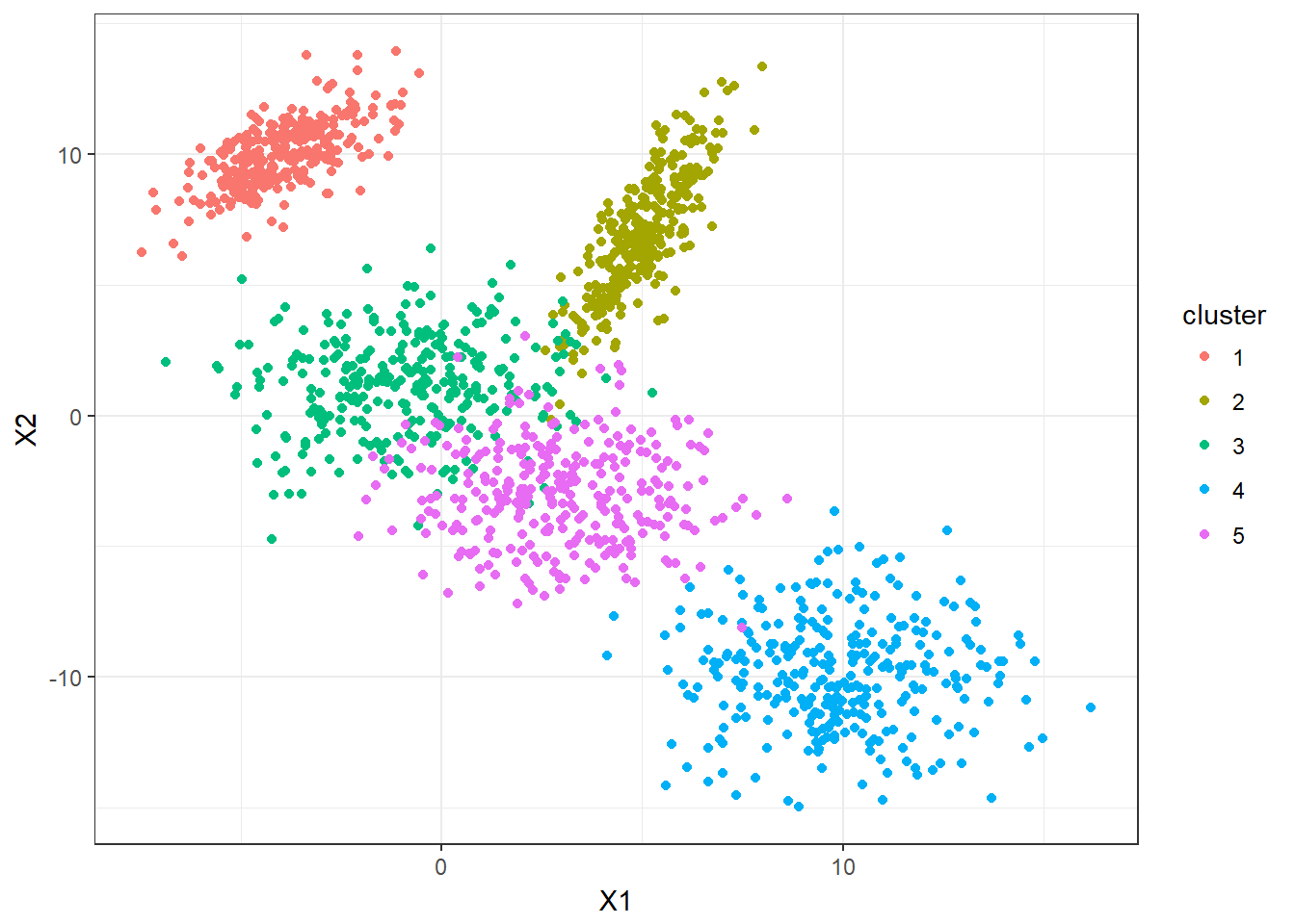
Now, let’s apply the K-means clustering function that we just defined. We can also visualize how K-means is performing in this dataset.
k = 5
res=mykmeans(DF[1:2],k=k)
res$centroid$cluster=1:k
res$data$isCentroid=F
res$centroid$isCentroid=T
data_plot2=rbind(res$centroid,res$data)

ggplot(data_plot2,aes(x=X1,y=X2,color=as.factor(cluster),
                           size=isCentroid,alpha=isCentroid)) +
  geom_point()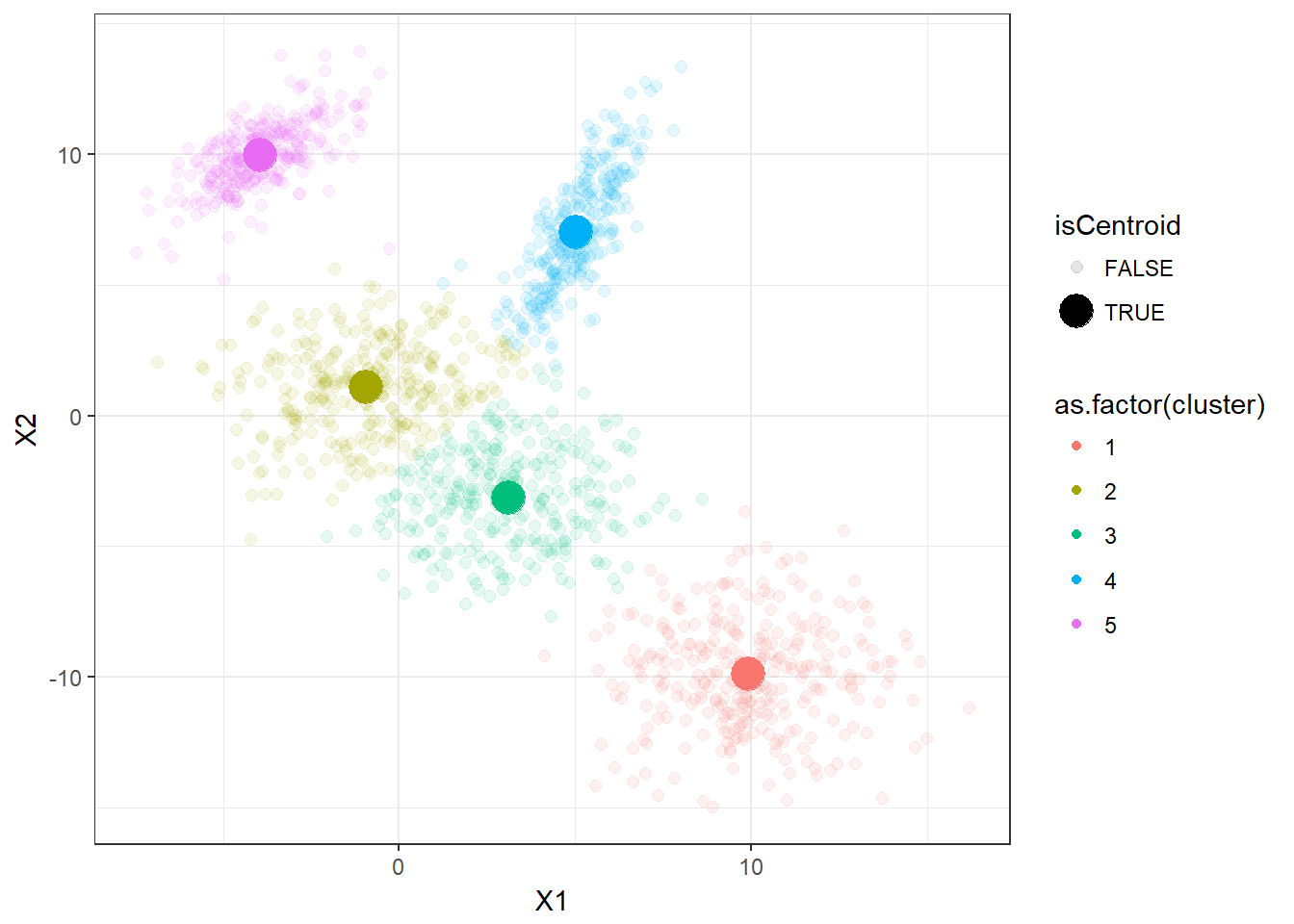
It appears that the K-means clustering is working well here since the 5 clusters are separated correctly.
Let’s look at how the K-means algorithm is working in the following visualization. We can see how the \(k = 5\) centroid is moving and form the 5 clusters correctly.
K-means ++ Clustering
The problem with k-means clustering is that it only provide local minimum but not global minimum. In other words, where you set as the inital centroids plays a big role. Thus, the usual method is to use different initial values, look for the stable solution (clusters) and choose the best initial value from there.
In 2007, David Arthur and Sergei Vassilvitskii introduced k-means++.
The big idea is that instead of choosing \(k\) centroids randomly, it’s better to choose the centroids such that they are far from each other. The major advantage of this approach is that we don’t have to try several initial values. This cuts down the computational time a lot.
The following is the algorithm of choosing the initial centroids:
- Denote a randomly chosen point as \(s_1\).
- For the \(l\) th iteration, \(l = 2,..., k\), compute the squared distances, \(D_i^2\): \[D_i^2 = min \{||Y_i -s_1||^2,..., ||Y_i -s_{l-1}||^2 \}\]. The probability that \(Y_i\) is chosen as the centroid, \(s_l\), is \[D_i^2/\sum_{j}D_j^2\] with \(i \neq j\) and \(i, j = 1,..., n\).
- Repeat this until we collect \(s_1, ..., s_k\).
- Use the collected points as the staring centroids for k-means algorithm.
Implementations
kmeanplus <- function(data, k, ...)
{
  n = nrow(data)

  # Place holder
  centroids <- rep(NA, k)
  dist <- matrix(nrow = n, ncol = k-1)

  # Initialize probability = 1 for all data points
  probs = rep(1, n)

  for (i in 1: (k-1))
  {
    # The s_k
    centroids[i] = sample.int(n, 1, prob = probs)
    # The D_i^2
    dist[,i] = (apply(data, 1, function(x) sum((x- data[centroids[i], ])^2)))
    # Not counting the exact probabily here. All we care is the relative weight.
    probs = apply(dist, 1, function(y) y[which.min(y)])
  }
  centroids[k] = sample.int(n, 1, prob = probs)

  res <- mykmeans(data = data, centers = centroids,  k = k, ...)
  return(res)
}
Visualization
Let’s reuse the same dataset as above and visualize the clustering process.
res <- kmeanplus(DF[1:2], k = 5)
The number of iterations is 7 this time.
Choosing K - the Elbow Method
The Elbow Method will be used in this case. Recall that all we were doing is to minimize the within cluster sum of squares. We can vary the value of \(k\), say from 3 to 7, and plot the within sum of squares against the \(k\) s. The location of a bend in the plot can be considered as the optimal \(k\) because it means that further increasing number of \(k\) is not decreasing the within sum of squares a lot.
set.seed(1001)

# Compute and plot wss for k = 3 to k = 7
k.values <-3:7

wss = c()

for (k in k.values)
{
  wss = c(wss, kmeanplus(DF[1:2], k = k)$tot.withinss)
}

plot(k.values, wss,
       type="b", pch = 19, frame = FALSE,
       xlab="Number of clusters K",
       ylab="Total within-clusters sum of squares",
       col = "dodgerblue")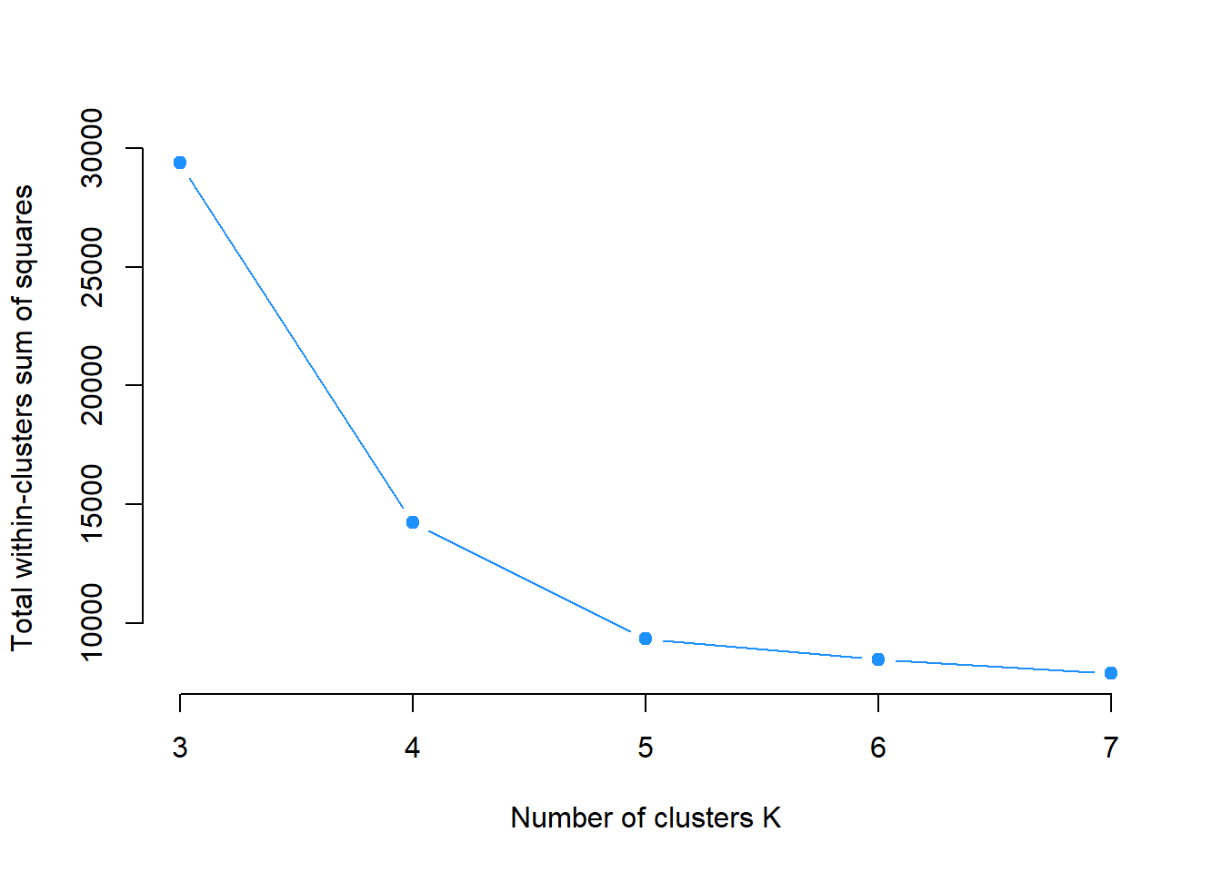
The Elbow is seen at \(k = 5\) and that is congruent with our simulated 5 clusters.
Next Step
There are different ways of choosing the number of clusters \(k\) in adddition to the Elbow method. One can also try on more data simulations and discover the limitations of k-means clustering.